Maxwell's Equations

Maxwell's Equations using System International (SI) units are shown in Table 1-1 in both differential or 'point' form and integral form [2]. In Section 2 we will see that the integral forms may be derived from the point forms using familiar vector identities. They also use the vector operators divergence (\(\nabla \bullet\)), curl (\(\nabla \times\)) and dot product (\( \bullet \)), as well as standard calculus operators and symbols, many of which had not been invented at the time of Maxwell [1] [3] [4] [6] [7] [8]. To avoid any inconsistency by simply numbering the equations, we will use the alternative names shown in the right-hand column. These relate the equations to the names of the scientists (Gauss, Faraday and Ampere) who also made significant discoveries and contributions to knowledge about electric and magnetic fields around the time of Maxwell (1831 - 1879).

Some earlier forms of Maxwell's equations, before SI units were widely adopted, were based on the centimetre-gram-second (CGS) system of units. In any references, if you see unexpected factors of \(4 \, \pi\) or \(c\) (the 'velocity of light'), bear in mind that you may be using the Heaviside-Lorentz or Gaussian variations.

To study Maxwell's Equations in their original form (some 20 equations and 20 variables) would have made a rather lengthy article, so we acknowledge the contributions to Maxwell's work from Heaviside (1850 - 1925), a self-taught mathematician and physicist. Heaviside developed a form of vector calculus which is widely used today and applied this to simplify Maxwell's work into their iconic form which we see in Table 1-1 [2].

Table 1-1 Maxwell's Equations in Differential Form

Maxwell (Differential Form)	Maxwell (Integral Form)	Alternative Name
\[\nabla \bullet \boldsymbol{E}=\frac{\rho}{\epsilon_0}\]	\[ {\Huge \unicode{x222F}_{\normalsize S }} \boldsymbol{E} \bullet d \boldsymbol{S} = \frac{1}{\epsilon_0} \iiint_V \rho \, d V \]	Maxwell-Gauss (Electric)
\[\nabla \bullet \boldsymbol{B}=0\]	\[ {\Huge \unicode{x222F}_{\normalsize S}} \boldsymbol{B} \bullet d \boldsymbol{S} = 0 \]	Maxwell-Gauss (Magnetic)
\[\nabla \times \boldsymbol{E}=-\frac{\partial \boldsymbol{B}}{\partial t}\]	\[ \oint_C \boldsymbol{E} \bullet d \boldsymbol{l} = -\frac{\partial}{\partial t} \iint_S \boldsymbol{B} \bullet d \boldsymbol{S} \]	Maxwell-Faraday (Induction)
\[\nabla \times \boldsymbol{H}=\boldsymbol{J} + \frac{\partial \boldsymbol{D}}{\partial t}\]	\[ \oint_C \boldsymbol{B} \bullet d \boldsymbol{l} = \mu_0 \iint_S \boldsymbol{J} \bullet d \boldsymbol{S} + \mu_0 \epsilon_0 \frac{\partial}{\partial t} \iint_S \boldsymbol{E} \bullet d \boldsymbol{S} \\ \]	Maxwell-Ampere (with Displacement Current Density)

The two Gauss forms and the Faraday equation were not changed by Maxwell from their originals. However, the Maxwell-Ampere equation results from Maxwell's amendment to Ampere's original (static) field version, to add the displacement current density term \( \left( \frac{\partial \boldsymbol{D}}{\partial t} \right) \). Although largely unrecognised at the time, this simple addition enabled the mathematical derivation of the wave equations to describe the propagation of electromagnetic waves. This will be described in Section 3.

All of Maxwell's equations apply to three dimensional space which is isotropic. This means that the scalar electromagnetic parameters for the medium containing the fields: conductivity (\(\sigma\)), permittivity (\(\epsilon\)) and permeability (\(\mu\)), are not functions of direction (\(x\), \(y\) and \(z\) if we choose the common rectilinear system). To start with, our assumption is that the medium is the simplest isotropic form available: a vacuum or 'free space'.

Scientists, engineers and mathematicians almost universally agree that Maxwell's equations apply everywhere. Of course, it is difficult to prove this, but in the 150 years or so since Maxwell, there have been many attempts to find exceptions to 'everywhere', so far without success. To date, the longest radio communication distance, using hardware designed according to Maxwell's equations, is about \(23 \times 10^{9} \, km \). This was between the Earth and the Voyager 1 spacecraft. The propagation time for the radio waves in each direction was approximately 21 hours. That was consistent with one of Maxwells conclusions, that radio waves travel at the speed of light in a vacuum.

The vector and scalar symbols and units used in Maxwell's Equations are defined below, together with their SI units.

• \(\boldsymbol{D}\): electric displacement field, surface charge density or electric flux density in coulombs per metre squared (\(C/m^2\)).
• \(\boldsymbol{B}\): magnetic flux density in tesla (\(T\)) or webers per metre squared (\(Wb/m^2\)).
• \(\boldsymbol{E}\): electric field in volts per metre (\(V/m\)).
• \(\boldsymbol{H}\): magnetic field in amperes per metre (\(A/m\)).
• \(\boldsymbol{J}\): current density in amperes per metre squared (\(A/m^2\)).
• \(\rho\): volumetric charge density in coulombs per metre cubed (\(C/m^3\)).
• \(\epsilon_0\): vacuum (free space) permittivity, \(8.85 \times 10^{-12} \) farads per metre (\(F/m\)).
• \(t\): time in seconds (\(s\)).

Although non-SI unit conventions still persist in electromagnetics, we will only be using SI units. We will also keep with our convention of using bold type-face symbols for vectors (such as \(\boldsymbol{E}\) and \(\boldsymbol{H}\)), and normal type-face symbols for scalars (such as \(\rho\) and \(t\)). For consistency, a three dimensional rectangular (\(x\), \(y\), \(z\)) co-ordinate system will be chosen, although any three dimensional co-ordinate system could be used with the necessary conversions.

Integration Methods

In Table 1-1, the letters \(V\), \(S\) and \(C\) used as subscripts for the integral symbols represent 'volume', 'surface' (area) and 'contour' respectively. These are described in the following paragraphs with the help of Figure 1-1 and Figure 1-2. Do not mistake this \( V \) for anything associated with voltage.

The Volume Integral \(\iiint_V\)

The volume integral used in the Maxwell-Gauss (Electric) equation is a three dimensional (triple) integral defining a closed volume which must be smooth without any holes. This will be the medium which will contain charges, positive or negative. Large and/or complex shapes will normally be reduced to combinations of small, regular shapes before processing.

The Surface Integrals \(\unicode{x222F}_S\) and \(\iint_S\)

The surface integral may be either a closed form, with a ring as part of the symbol, or a double integral which applies across a defined boundary. The closed form may be described with the help of Figure 1-1.

The surface shown represents an arbitrary volume \(V\) enclosed within a smooth surface \(S\) with no holes. The infinitesimal integration method will reduce \(V\) to the point under consideration at \(P\). \(V\) is located within the generic vector field which we will call \(\boldsymbol{F}\). \(\boldsymbol{F}\) may be any vector field encountered in electromagnetics, for example electric field \(\boldsymbol{E}\) or magnetic field \(\boldsymbol{H}\). In general \(\boldsymbol{F}\) is assumed to be non-uniform and could therefore be represented at any defined point by its three dimensional components such as \(\boldsymbol{F} = F_x \; \hat{\boldsymbol{x}} + F_y \; \hat{\boldsymbol{y}} + F_z \; \hat{\boldsymbol{z}}\). Here, \(\hat{\boldsymbol{x}}\), \(\hat{\boldsymbol{y}}\) and \(\hat{\boldsymbol{z}}\) are the unit vectors in the \(x\), \(y\) and \(z\) directions respectively, also \(F_x\), \(F_y\) and \(F_z\) represent their respective component magnitudes.

We will consider the integration operator applied at the point \(P\) on \(S\), but the same arguments may be applied at any point on the surface. The surface area infinitesimal element is the scalar value \(d S \). The surface may contain any combination of regions which are concave, convex or saddle type. In this example, point \(P\) happens to be concave but it could be any type. Some normal unit vectors \( \boldsymbol{\hat{n}} \) are also shown in the area \(d S \). As the integration limit is approached, these will reduce to just one normal vector at point \(P\), at which \(d S\) is considered to still be finite but very close to zero, when it becomes a small tangential plane. A 'magnified' form of this is illustrated in Figure 1-2.

In the limit, as there will be just one normal vector \(\boldsymbol{\hat{n}}\) at \(P\), the vector field will also have just one value \(\boldsymbol{F}\) as shown, say at an angle \(\theta\) to \(\boldsymbol{\hat{n}}\). As \(\boldsymbol{\hat{n}}\) is normal to the plane \(d S\) and has a magnitude of one by definition, the dot product \(\boldsymbol{F} \bullet \boldsymbol{\hat{n}} \) will be the component of \(\boldsymbol{F}\) normal to the plane at that point, \(F \cos{\theta}\). This relationship is often useful if we require to calculate flux magnitudes passing normally through surfaces at various points. For example, if \(\boldsymbol{F}\) was magnetic flux density \(\boldsymbol{B}\) in units of tesla (\(T\)) or webers per metre squared (\(Wb /m^2\)), then the dot product would yield the normal component of \(\boldsymbol{B}\) at \(P\). The scalar product of this and the tangential area would give the total magnetic flux in webers in the normal direction. The surface vector \(d \boldsymbol{S} \) is the product of the normal unit vector \(\boldsymbol{\hat{n}}\) and the scalar area \(d S\). We will often encounter similar dot products in the electromagnetics equations.

The double integral form of surface integral is again used to calculate an area, but not the area of a closed surface. The actual area would be defined using limits appropriate to the geometry of the practical case under consideration.

The Contour Integral \(\oint_C\)

The contour integral is a form of line integral or path integral applied along the path of a closed contour \(C\) on a smooth surface. The path may take any route in three dimensions provided it is continuous.

Isotropic Material Properties

Apart from the electric and the magnetic fields, there are three other vector fields central to Maxwell's equations: current density \(\boldsymbol{J}\) (1.2-1), displacement field \(\boldsymbol{D}\) (1.2-2) and magnetic flux density \(\boldsymbol{B}\) (1.2-3). Each of these which may be derived from the electric field (\(\boldsymbol{E}\)) or the magnetic field (\(\boldsymbol{H}\)) using the properties of conductivity, permittivity or pearmeability.

\[ \boldsymbol{J}=\sigma \boldsymbol{E} \]

\[ \boldsymbol{D}=\epsilon \, \boldsymbol{E} = \epsilon_0 \, \epsilon_r \, \boldsymbol{E} \]

\[ \boldsymbol{B}=\mu \boldsymbol{H} = \mu_0 \, \mu_r \, \boldsymbol{H} \]

The scalar coefficients used in (1.2-1), (1.2-2) and (1.2-3) are described below.

• \(\sigma\): conductivity in siemens per metre (\(S/m\)).
• \(\epsilon\) (= \(\epsilon_0 \, \epsilon_r\)): permittivity in farads per metre (\(F/m\)).
• \(\epsilon_0\): vacuum (free space) permittivity in farads per metre (\(F/m\)).
• \(\epsilon_r\): relative permittivity, also known as dielectric constant (unitless).
• \(\mu\) (= \(\mu_0 \, \mu_r\)): permeability in henries per metre (\(H/m\)).
• \(\mu_0\): vacuum (free space) permeability in henries per metre (\(H/m\)).
• \(\mu_r\): relative permeability (unitless).

In SI Units \(\epsilon_0 \, = \, 8.85 \times 10^{-12} \, F/m \) and \(\mu_0 \, = \, 4 \pi \times 10^{-7} \, H/m \) [2].

In this article we are only considering isotropic media, so the coefficients for conductivity, permittivity and permeability are assumed to be scalars. Furthermore, for free space, both the relative permittivity and the relative permeability are unity and therefore a real value by definition, so \(\epsilon = \epsilon_0 \) and \(\mu = \mu_0 \). However, it is interesting to note that, under certain conditions \(\sigma\), \(\epsilon\) and \(\mu\) can be mathematically represented by complex values. Further information is available from the following Wikipedia articles.

• Complex conductivity.
• Complex permittivity.
• Complex permeability.

The Integral Forms of Maxwell's Equations

In the following sub-sections we will take the point forms of Maxwell's equations listed in Table 1-1 and convert each of them to the associated integral form using the Divergence Theorem (2-1) and Stokes Theorem (2-2).

\[ \begin{align} \iiint_V \nabla \bullet \boldsymbol{F} \, \mathrm{d} V &= {\Huge \unicode{x222F}_{\normalsize S}} \boldsymbol{F} \bullet \boldsymbol{\hat{n}} \,\mathrm {d} S \\ &= {\Huge \unicode{x222F}_{\normalsize S}} \boldsymbol{F} \bullet d \boldsymbol{S} \\ \end{align} \]

\[ \iint _{S} \nabla \times \boldsymbol{G} \, \bullet d \boldsymbol{S} = {\Huge \unicode{x222F}_{\normalsize C}} \boldsymbol{G} \bullet d \boldsymbol{l} \]

More information on these theorems are included in the article on vector operators and theorems.

The Maxwell-Gauss (Electric) Equation (2.1-1)

\[\nabla \bullet \boldsymbol{E}=\frac{\rho}{\epsilon_0}\]

Using (1.2-2), this may be expressed as the divergence of a displacement field (2.1-2).

\[\nabla \bullet \boldsymbol{D}=\rho\]

This is the differential form of the Maxwell-Gauss (Electric) equation. We may express this in the integral form using the Divergence Theorem (2-1).

There are two types of charge distribution to consider, the displacement field, also known as surface charge density, which is a vector (\(\boldsymbol{D}\)) and the volumetric charge density (\(\rho\)) which is a scalar. The SI units for these are coulombs per metre squared \( \left( C/m^2 \right) \) and coulombs per metre cubed \( \left( C/m^3 \right) \) respectively.

The Divergence Theorem may be applied to (2.1-2) by replacing \( \boldsymbol{F} \) by \(\boldsymbol{D}\). This yields the Maxwell-Gauss (Electric) equation in integral form (2.1-3).

\[ \begin{align} \iiint_V \nabla \bullet \boldsymbol{D} \, d V &= {\Huge \unicode{x222F}_{\normalsize S}} \boldsymbol{D} \bullet \boldsymbol{\hat{n}} \, d S \\ &= {\Huge \unicode{x222F}_{\normalsize S}} \boldsymbol{D} \bullet d \boldsymbol{S} \\ \iiint_V \rho \, d V &= {\Huge \unicode{x222F}_{\normalsize S}} \boldsymbol{D} \bullet d \boldsymbol{S} \\ {\Huge \unicode{x222F}_{\normalsize S}} \boldsymbol{E} \bullet d \boldsymbol{S} &= \frac{1}{\epsilon_0} \iiint_V \rho \, d V \\ \end{align} \]

Equations like those in (2.1-3) require some careful use of the correct symbols for bold-font (vectors) and normal-font (scalars and operators). On the first line we have \(\hat{\boldsymbol{n}}\) which is the unit vector in the normal direction for the elementary (scalar) surface area \(d S\). As we noted in Section 1.1.2, at the limit of integration, the (simple) product \(\boldsymbol{\hat{n}} \, d S\) is that of a scalar \(d S \) and a vector \(\boldsymbol{\hat{n}}\), so the result is a vector \( d \boldsymbol{S} \) known as a vector area or 'orientated vector (2.1-4).

\[ \boldsymbol{\hat{n}} \, d S = d \boldsymbol{S} \]

The Maxwell-Gauss (Magnetic) Equation (2.2-1).

\[\nabla \bullet \boldsymbol{ B} = 0\]

To obtain the integral form we need to again apply the Divergence Theorem, using the same equation that was used for the Maxwell-Gauss (Electric) equation in Section 2.1 (2.1-3). This one is easier (2.2-2). Again, this also uses the vector area relationship .

\[ \begin{align} \iiint_V \nabla \bullet \boldsymbol{B} \, d V &= {\Huge \unicode{x222F}_{\normalsize S}} \boldsymbol{B} \bullet \boldsymbol{\hat{n}} \, d S = 0 \\ {\Huge \unicode{x222F}_{\normalsize S}} \boldsymbol{B} \bullet d \boldsymbol{S} &= 0 \\ \end{align} \]

The Maxwell-Faraday Equation (2.3-1)

\[ \nabla \times \boldsymbol{E}=-\frac{\partial \boldsymbol{B}}{\partial t} \]

As this includes the curl vector operator (\( \nabla \times \)), to express it in integral form we may use Stokes Theorem (2-2). The result is the Maxwell-Faraday equation in integral form (2.3-2).

\[ \begin{align} \iint_S \nabla \times \boldsymbol{E} \bullet d \boldsymbol{S} &= \oint_C \boldsymbol{E} \bullet d \boldsymbol{l} \\ &= -\frac{\partial}{\partial t} \iint_S \boldsymbol{B} \bullet d \boldsymbol{S} \\ \oint_C \boldsymbol{E} \bullet d \boldsymbol{l} &= -\frac{\partial}{\partial t} \iint_S \boldsymbol{B} \bullet d \boldsymbol{S} \\ \end{align} \]

The Maxwell-Ampere Equation (2.4-1)

\[ \nabla \times \boldsymbol{H}=\boldsymbol{J} + \frac{\partial \boldsymbol{D}}{\partial t} \]

Using a similar method to that used for the Maxwell-Faraday equation, we may again use Stokes Theorem (2-2) to change this to the integral form (2.4-2). This one is a little more difficult, so I have added a few extra lines which you will hopefully be able to confirm.

\[ \begin{align} \nabla \times \boldsymbol{H} &= \boldsymbol{J} + \frac{\partial \boldsymbol{D}}{\partial t} \\ \iint_S \nabla \times \boldsymbol{H} \bullet d \boldsymbol{S} &= \oint_C \boldsymbol{H} \bullet d \boldsymbol{l} \\ \oint_C \boldsymbol{H} \bullet d \boldsymbol{l} &= \iint_S \left(\boldsymbol{J} + \frac{\partial \boldsymbol{D}}{\partial t} \right) \bullet d \boldsymbol{S} \\ &= \iint_S \boldsymbol{J} \bullet d \boldsymbol{S} + \frac{\partial}{\partial t} \iint_S \boldsymbol{D} \bullet d \boldsymbol{S} \\ \frac{1}{\mu_0} \oint_C \boldsymbol{B} \bullet d \boldsymbol{l} &= \iint_S \boldsymbol{J} \bullet d \boldsymbol{S} + \epsilon_0 \frac{\partial}{\partial t} \iint_S \boldsymbol{E} \bullet d \boldsymbol{S} \\ \oint_C \boldsymbol{B} \bullet d \boldsymbol{l} &= \mu_0 \left[ \iint_S \boldsymbol{J} \bullet d \boldsymbol{S} + \epsilon_0 \frac{\partial}{\partial t} \iint_S \boldsymbol{E} \bullet d \boldsymbol{S} \right] \\ \end{align} \]

Maxwell's Modification to Ampere's Circuital Current Law [8]

Except for updated mathematical symbology, the Maxwell-Gauss and Maxwell-Faraday equations shown in Table 1-1 are unchanged from their original forms discovered by Gauss and Faraday. However, the Maxwell-Ampere equation was modified by Maxwell from Ampere's original 'Circuital Current Law' by adding the second (time varying or \(\partial t \) operator) term on the right-hand side for both the point form and the integral form. The respective forms of the Ampere's original Circuital Current Law, before modification by Maxwell, are shown in (3-1) and (3-2).

\[\nabla \times \boldsymbol{H}=\boldsymbol{J} \]

\[\oint_C \boldsymbol{B} \bullet d \boldsymbol{l} = \mu_0 \iint_S \boldsymbol{J} \bullet d \boldsymbol{S} \]

Around Maxwell's time, it was known that condensers, the predecessors of the parts we now call capacitors, were formed by two conductive plates separated by a thin insulator, and were capable of storing charge. Faraday had also demonstrated the properties of magnetic flux linkage between coils and magnets but only on condition that the flux was changing. It was also known that electrical current passed along wires: long thin conductors, but it did not pass through insulators. How then did some sort of electric current appear to 'jump' across the air gaps between between coils and magnets or across the capacitor plates? If it could jump a few inches in this way, could it jump rather longer distances such as those between towns or even countries? That would be very useful. The following thought experiment describes Maxwell's reasoning that Ampere's Circuital Current Law was inadequate for time varying fields.

Figure 3-1 shows a circuit using modern schematic symbols designed to charge the air-spaced capacitor \(C\), considered to have circular, parallel plates, from a battery \(B\) through a resistor \(R1\) when the switch \(SW1\) is in position \(1\). Once the capacitor is fully charged, the switch may be moved to position \(2\), allowing it to dischage through another resistor \(R2\). The capacitance and resistor values must be chosen to allow relatively slow charge and discharge times to approximate to static field conditions. Maxwell considered Ampere's Circuital Law (3-2) applied at two positions on a practical circuit of this type.

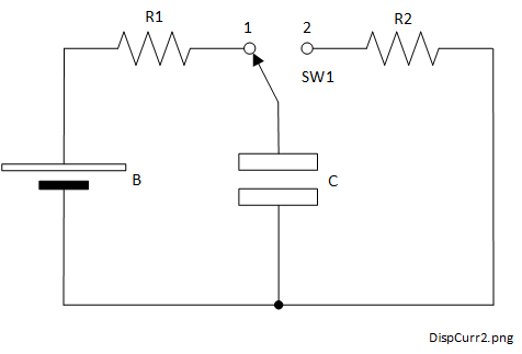
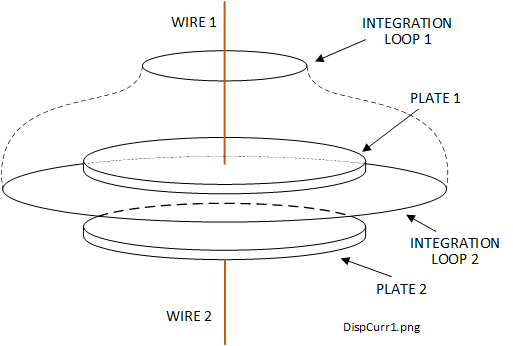
Figure 3-2 shows a section of such a circuit near the capacitor, including the parallel circular plates and a wire connection to each plate (WIRE1 and WIRE 2) to connect to the rest of the circuit.

When \(C\) charges, current flows, say in through WIRE 1 and out through WIRE 2, gradually reducing until it reaches zero when \(C\) becomes fully charged. When \(SW1\) is switched to position 2, it discharges through \(R2\) starting with a high current and gradually reducing to zero when \(C\) becomes discharged again.

Ampere's Circuital Law (3-2) applied around one of the wires, say WIRE 1 at INTEGRATION LOOP 1, as shown in Figure 3-2 , was found to give the expected result for the magnetic flux density. However, applying it again at INTEGRATION LOOP 2, including the condenser dielectric, predicted a magnetic flux density of zero as it includes the capacitor dielectric which is an insulator. An insulator conducts zero current so the current density \(\boldsymbol{J} \) must also be zero. So how could the magnetic field generated by the current be finite and zero at different parts of the same circuit?

In an attempt to solve this anomoly, Maxwell added the time varying term \(\partial{\boldsymbol{D}} / \partial t \) to the point form of Ampere's Circuital equation. \(\boldsymbol{D}\) is the electric displacement field due to the polarisation effects observed in capacitors when they are charged and has units of surface charge density in coulombs per metre squared (\(C/m^2\)). The current density resulting from \(\partial{\boldsymbol{D}} / \partial t \), had the same units as conduction current density \(\boldsymbol{J}\) in ampere per metre squared (\(A/m^2\)). This became known as displacement current density. to distuinguish it from (conduction) current density. Conduction current is caused by moving charges within a conductor. Displacement current originates from the changes in electric field across a dielectric such as the capacitor in this example.

Conclusion

Time Dependence

Neither the electric nor magnetic forms of the Maxwell-Gauss equations includes the time (\(t\)), so these apply only to static, or non-time varying fields. Static fields are generated by direct current (DC). DC may alternatively be described as an alternating current (AC) at zero frequency. In the many years since Maxwell we have learnt that we may sometimes approximate finite but 'low frequency' AC to DC. In most cases this is valid provided that the dimensions of the electrical parts of the circuit under consideration are a very small fraction of a free space wavelength. For example, common power transmission frequencies for AC are 50 Hz, 60 Hz and 400 Hz. The associated free space wavelengths are 6000 km, 5000 km and 750 km respectively. Therefore, if the electrical parts (wires, capacitors, switches etc.) have dimensions in the order of a few metres, the static approximation will hold.

The Maxwell-Faraday and Maxwell-Ampere equations both contain the partial differential operator applied to time (\(\partial t\)). Faraday's experiments on electromagnetic induction found that the apparent amplitude of the induced current depended on a change in the magnitude of the magnetic flux linking the magnet and coil. This made it a function with a time-varying property. For the Maxwell-Ampere equation, the right-hand side of both the point and integral forms contain two terms as shown in Table 1-1. In each case the first is the original static case term discovered by Ampere. As we noted, the second was introduced by Maxwell to account for what was described as a 'displacement current density': a current generated by a changing electric field rather than moving charges charges as described in Section 3. Although not appreciated by many at that time, this made the first formal mathematical connection between electric fields, magnetic fields and time and was a revolutionary breakthrough in electromagnetics [8]. Maxwell used this relationship to mathematically prove the existence of electromagnetic waves capable of propagating through any non-conducting medium, including free space, at or near the speed of light.

The Historical Perspective

Maxwell's mathematical breakthrough provided the long awaited links between magnetic fields, electric fields and time. It enabled the derivation of a set of second order differential equations which could be solved simultaneously. This proved that plane, polarised electromagnetic waves can propagate through both free space and loss-free dielectric media at or near the speed of light. Furthermore, light itself was simply an optical subset of electromagnetic waves obeying exactly the same equations. Before Maxwell, optical methods had been used to predict the speed of light to reasonable accuracy without using its electric or magnetic field properties. Maxwell was able to link these, respectively the free space values of permittivity \(\epsilon_0\) and permeability \(\mu_0\), by a simple equation to produce a value for the speed of electromagnetic radiation in free space, \(c\, = \,1 / \sqrt{\epsilon_0 \mu_0}\).

Modern references to Maxwells Equations benefit from over 150 years of attempts to prove them wrong, so far without success. At Maxwell's time there was significant knowledge about the properties of electric and magnetic fields and many experiments had been conducted by Faraday, Ampere, Gauss and many other scientists. Their results are still valid today for static fields and many very low frequency fields. However, Maxwell's work provided the theory to enable the propagation of what we now refer to as radio waves or wireless communications.

The Heaviside 'Simplification' and Vector Calculus

Maxwell's original presentation of his now famous equations were in a more verbose form, including some 20 separate equations using 20 varaibles. A few years' later, Heaviside's mathematical contribution was to combine them into just the 4 'simplified' equations using vector operators which he had invented and calculus notation. Stokes Theorem and the Divergence Theorem, based on Gauss's work were used to development them into the point and integral forms which are popular today.

The Maxwell-Gauss (Electric) Equation (4.4-1) and (4.4-2)

\[\nabla \bullet \boldsymbol{E}=\frac{\rho}{\epsilon_0}\]

\[ {\Huge \unicode{x222F}_{\normalsize S }} \boldsymbol{E} \bullet d \boldsymbol{S} = \frac{1}{\epsilon_0} \iiint_V \rho \, d V \]

What does the Maxwel-Gauss (Electric) equation mean? The definition of the divergence operator (\(\nabla \bullet\)) applied to the electric field vector \( \boldsymbol{E} \) expressed in rectangular (\( x, \, y, \, z \, \)) co-ordinates is shown in (4-2).

\[ \nabla \bullet \boldsymbol{E} = \frac{\partial E_x}{\partial x} + \frac{\partial E_y}{\partial y} + \frac{\partial E_z}{\partial z} \]

The result is a scalar. (4-2) shows this to be the sum of the magnitudes of the (spatial) rates of change of the rectangular components of \(\boldsymbol{E}\). As its name would imply, application of the divergence operator to a vector field is a measure of its 'outgoingness'. That is, how much at the point of measurement, the vectors either flow out of an apparent source or towards an apparent sink. The most popular convention and that assumed for Maxwell's equations is to use a positive divergence result for a source and a negative value for a sink. Therefore, the Maxwell-Gauss (Electric) equation tells us that, for a positive divergence result at a point, the result is the volumetric charge density divided by the free space permittivity, \( \epsilon_0 \) (4-3).

\[ \frac{\partial E_x}{\partial x} + \frac{\partial E_y}{\partial y} + \frac{\partial E_z}{\partial z} = \frac{\rho}{\epsilon_0}\]

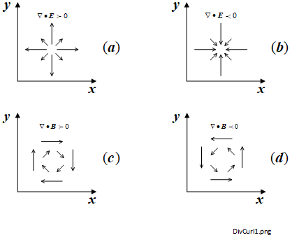
Figure 4-1 (a) and (b) shows a simplified, two dimensional (\(x , \,y\)) depiction of some electric field vectors for \(\nabla \bullet \boldsymbol{E} \gt 0 \) and \(\nabla \bullet \boldsymbol{E} \lt 0 \) respectively. Each arrows' direction and length represent the vector field direction and magnitude at that point. The magnitude of the divergence result determines the magnitude of the positive or negative charge respectively.

It also also tells us that, using our convention, for every (positive) source charge there must somewhere be an equivalent negative sink charge to imply the existence of the electric field. The next is usually: what happens if the divergence result is zero? Well, it is not here by definition but, for the Maxwell-Gauss (Magnetic Field) equation, it is. You will be interested to read about that in Section 4.5.

The Maxwell-Gauss (Magnetic) Equation (4.5-1) and (4.5-2)

\[\nabla \bullet \boldsymbol{B} = 0 \]

\[ {\Huge \unicode{x222F}_{\normalsize S}} \boldsymbol{B} \bullet d \boldsymbol{S} = 0 \]

Just as we saw in Section 4.4 for the Maxwell-Gauss (Electric) equation, the definition of the divergence vector operator (4-2) may also be used for the Maxwell-Gauss (Magnetic) equation (4-4). In this case the divergence result is (defined to be) zero. The magnetic vector fields will therefore take up the shapes of loops similarly to those shown in Figure 4-1 (c) and (d). The directions of the fields within the loops will be determined by the direction of the magnetic field according to a definition such as a 'left-hand' or 'right-hand' rule.

So in magnetic fields, we are talking about 'directional, continuous loops of flux density' rather than sources and sinks of the type we discovered for electric fields. Any device which generates a magnetic field, such as an permanent magnet or an electro-magnet will generate such fields in the form of loops. The loops can however be distorted and re-routed by nearby magetic devices. The biggest natural magnetic phenomenon at the time of Maxwell was the Earth's magnetic field. Versions of the navigational compass were invented well before Maxwell. The tendancy of these to align with the Earth's magnetic field allowed the definition of the magnetic field direction as either 'north seeking' (N) or 'south seeking' (S) and compass needles which were effectively small bar magnets, were marked accordingly. We know that magnetic fields are formed in loops. Therefore a complete magnetic flux loop may be considered to comprise a series of small bar magnets each orientated with its N pole next to the S pole of the next magnet.

The Maxwell-Faraday Equation (4.6-1) and (4.6-2)

\[\nabla \times \boldsymbol{E}=-\frac{\partial \boldsymbol{B}}{\partial t}\]

\[\oint_C \boldsymbol{E} \bullet d \boldsymbol{l} = -\frac{\partial}{\partial t} \iint_S \boldsymbol{B} \bullet d \boldsymbol{S} \]

The Maxwell-Faraday equation is unchanged from Faraday's original form, except for the use of 'modern' vector and calculus operators. Faraday's Law of Electromagnetic Induction applied to the interaction of magnetic fields and nearby coils formed of conducting wires. Two of his well known experiments are shown schematically in Figure 4-2 (a) and (b).

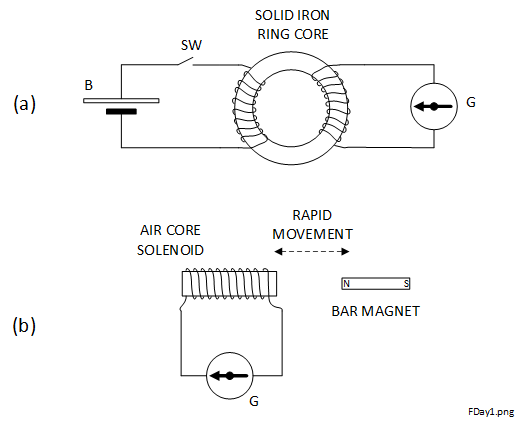
In (a), a battery \(B\) was connected to one coil, formed of insulated wire, wound around an iron ring core via a switch \(SW\). A galvanometer \(G\) (an instrument for measuring small currents) was connected to a similar second coil wound on the same ring. Whilst \(SW\) was open for a long time or closed for a long time, there was no deflection from the needle of \(G\). At the instant of closing \(SW\) a pulse was was observed on \(G\). Similarly a pulse, but in the opposite direction, was observed on \(G\) when opening \(SW\), if it had previously been closed for a long time. These observations were consistent with the results of experiments by Emil Lenz and Joseph Henry. During similar experiments, Lenz and Henry found that the induced current acted in a direction so as to oppose the direction of the field causing it. We would recognise the similarity of Faraday's parts with the modern transformer. Faraday changed the number of turns of the sensing coil and noted with some surprise 'an increased deflection of the galvanometer with fewer turns', of course entirely consistent with today's understanding of 'turns-ratio'.

In (b), the degree of 'linking' of a magnetic field from a permanent 'bar' magnet to a solenoid coil was changed by moving it in and out of the solenoid air-core. If there was no relative movement between the magnet and solenoid the galvanometer did not deflect. If there was movement, the galvanometer recorded a deflection. The direction of the deflection and its magnitude varied according to the speed of the movement and its direction. The faster the movement the greater the deflection.

Faraday's two key conditions for demonstrating electromagnetic induction were:

• The source of the magnetic field, permanent magnet or electromagnet, had to be sufficiently close to the detection coil to allow the magnetic field to 'link' with it.
• The magnitude of the flux linkage had to be changed with respect to time.

To enable adequate linkage, the closeness of the magnetic field source (permanent magnet or electromagnet) required to be no more than a few inches from the sensing coil attached to the galvanometer. Clearly, this method was well short of working between towns or countries. The magnitude of the flux linkage could be changed with respect to time by physically moving the magnetic field source relative to the sensing coil. Alternatively, the electromagnet and the sensing coil could be positioned in close proximity at fixed positions. Then the current source could be switched on an off and pulses observed on the galvanometer only when the current was changing: either on to off or off to on.

Faraday's original experiments on electromagnetic induction were significant contributions to the development of today's motors, generators, solenoids, inductors and transformers. Although Maxwell's immediate interests were not motors and generators, he did believe Faraday's equation was mathematically correct. He used this together with Ampere's Circuital law, including the displacement current density term \( \left( \frac{\partial \boldsymbol{D}}{\partial t} \right) \). Faraday's work did not extend to the mathematical depth of Maxwell's.

The Maxwell-Ampere Equation (4.7-1) and (4.7-2)

\[\nabla \times \boldsymbol{H}=\boldsymbol{J} + \frac{\partial \boldsymbol{D}}{\partial t}\]

\[ \oint_C \boldsymbol{B} \bullet d \boldsymbol{l} = \mu_0 \iint_S \boldsymbol{J} \bullet d \boldsymbol{S} + \mu_0 \epsilon_0 \frac{\partial}{\partial t} \iint_S \boldsymbol{E} \bullet d \boldsymbol{S} \\ \]

The Maxwell-Ampere equation was the only one of the four Maxwell equations that was actually amended by Maxwell from it's original form, in this case Ampere's 'circuital law'. This was described in Section 3.

References

1. Pozar, David M.; Microwave Engineering, Third Edition; Wiley International Edition; John Wiley & Sons Inc.; Appendix B, pp 682-683: B1 (Dot Product), B2 (Cross Product), B12 (Divergence of a Curl = 0), B15 (Divergence Theorem), B16 (Stokes Theorem); ISBN 0-471-44878-8.
2. Pozar, David M. (op. cit.); Maxwell's Equations, applications of vector operators; pp 5-9.
3. Kreyszig, Erwin; Advanced Rngineering Mathematics, Fourth Edition; John Wiley & Sons, New York; pp 262-266 (Dot Product), pp 401-404 (Divergence of a Vector Field), pp 406-407 (Curl of a Vector Field), pp 444-448 (Divergence Theorem of Gauss), pp 454-457 (Stokes Theorem).
4. Kraus and Carver; Electromagnetics - Second Edition, International Student Edition; McGraw-Hill; pp 98-99 (Divergence Theorem), pp 93-97 (divergence of surface charge density), pp 98-99 (Divergence Theorem), pp 175-182 (Curl), pp 34-36 (Gradient); ISBN 0-07-035396-4.
5. Hayt, William H.; Engineering Electromagnetics, Fourth Edition; McGraw-Hill; pp 80-83 (Divergence Theorem), pp 75-78 (divergence definition), pp 254-261 (Curl), pp 106-112 (Gradient), pp 262-267 (Stokes' Theorem); ISBN 0-07-027395-2.
6. Ramo S., Whinnery J. R., Van Duzer, T.; Fields and Waves in Communication Electronics; John Wiley & Sons; pp 76-78 (Dot Product); pp 106-108 (Cross Product); p 85 (Divergence Theorem).
7. Griffiths, David J.; Introduction to Electrodynamics, Fourth Edition; Pearson Education Inc.; pp 2-3 (Dot Product), pp 3-4 (Cross Product); pp 34-36 (Stokes Theorem), pp 31-34 (Divergence Theorem), p 23, 24, 53, 243, 279 (Divergence of a curl is zero). ISBN 978-0-321-85656-2.
8. Feynman, Richard; The Maxwell Equations; The Feynman Lectures on Physics, Volume II, Chapter 18; California Institute of Technology, Michael A. Gottlieb and Rudolf Pfeiffer.