Important Vector Operators and Theorems for Electromagnetics

What are Vector Operators and Why Should We Get Familiar with Them?

In this article we are considering vectors in the context of vector fields as opposed to scalar fields. A vector field, such as an electric field (\(\boldsymbol{E}\)) or a magnetic field (\(\boldsymbol{H}\)), we will consider to exist in a volume, any position in which, may be described by rectangular (\(x,\,y,\,z\)) co-ordinates. For example, we could say that, at position \(P_1\), at co-ordinates (\(x_1 \,,y_1 \,,z_1\)), the magnetic field \(\boldsymbol{H_1}\) is given by \( \boldsymbol{H_1} = H_{1x} \, \boldsymbol{\hat{x}} + H_{1y} \, \boldsymbol{\hat{y}} + H_{1z} \, \boldsymbol{\hat{z}}\). Typically, as in this example, the local vector field values will be function(s) of their positions using the same co-ordinate system. This is recommended where possible for consistency. It is important to be able to distinguish between the (spatial) position at which the vector field is being measured and the components of the vector field itself at that point. Having said that, there are many different co-ordinate systems which may be used other than the rectangular. We will keep with the rectangular in this article.

Vectors are represented in magnitude and direction and are used extensively in science and engineering. Vector operators are short-hand methods for performing useful mathematical operations on vectors. As our particular interest is electromagnetics, \(\boldsymbol{E}\) and \(\boldsymbol{H}\) vectors will often be encountered, but there are many other vectors which are derived from these.

In general, we will assume 3 dimensional vector(s), such as \(\boldsymbol{A}\) represented using components directed along rectangular (\(x, \; y, \;z\)) directions and similarly for \(\boldsymbol{B}\) and so on. The unit vectors are defined \(\hat{\boldsymbol{x}}, \; \hat{\boldsymbol{y}}, \; \hat{\boldsymbol{z}} \) respectively. Therefore \(\boldsymbol{A} = A_x \; \hat{\boldsymbol{x}} + A_y \; \hat{\boldsymbol{y}} + A_z \; \hat{\boldsymbol{z}}\) where the magnitudes of the vector components in the \(x\), \(y\) and \(z\) directions are \(A_x \), \(A_y \) and \(A_z \) respectively. Note the convention we have adopted: bold typeface is used for vectors such as \(\boldsymbol{A}\) and \(\hat{\boldsymbol{x}}\) and normal typeface is used for scalars such as \( A_x \) and \( A_y \).

We try to consistently use Systeme International (SI) units. All of the vector and scalar parameters that we use in electromagnetics may be expressed in terms of the SI base units: mass (kilogram, kg), length (metre, m), time (second, s) and electric current (ampere, A). The other SI base units are amount of substance (mole, mol) and luminous intensity (candela, cd). Some parameters are unitless, for example relative permittivity or dielectric constant (\( \epsilon_r \)) and relative permeability (\( \mu_r \)), both of which are scalars. Several units are simplified by using other derived SI units such as the volt (\(V\)) and watt (\(W\)). Some examples are volts per meter (\(V / m\)) for electric field strength (\(\boldsymbol{E}\)), amperes per meter (\(A/m\)) for magnetic field strength (\(\boldsymbol{H}\)) and watts per square metre (\(W / m^2\)) for far field power flux density (\(\boldsymbol{S}\)). All of the vectors under consideration must be linearly related and scaled either to the same units or derived units.

We will look at the following vector operators and methods.

• Dot Product (\(\boldsymbol{A} \bullet \boldsymbol{B} \))
• Cross Product (\(\boldsymbol{A} \times \boldsymbol{B} \))
• Gradient Operator (\(\nabla A \))
• Divergence Operator (\(\nabla \bullet \boldsymbol{A} \))
• Curl Operator (\( \nabla \times \boldsymbol{A} \))
• Divergence Theorem
• The Divergence of a Curl is Zero Property
• Stokes Theorem

Dot Product

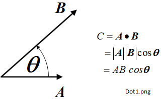
The dot product, say \(C\), of two vectors \(\boldsymbol{A}\) and \(\boldsymbol{B}\) is represented by the dot operator (\(\bullet\)), so \(C = \boldsymbol{A} \bullet \boldsymbol{B}\) [1] [3] [6] [7]. The result is a scalar, so \(C\) is represented in normal font. The definition of dot product of two vectors is the product of the vector magnitudes and the cosine of the (smaller) angle between them, measured in the same plane as the vectors (1.2-1). This is illustrated in Figure 1.2-1.

\[ C = \boldsymbol{A} \bullet \boldsymbol{B} = A \, B \, cos \, \theta \]

Cross Product

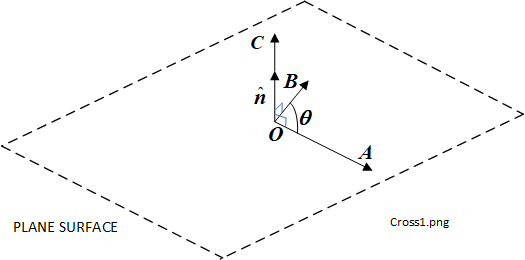
The cross product, say \(\boldsymbol{C}\), of two vectors \(\boldsymbol{A}\) and \(\boldsymbol{B}\) uses the cross (or times) operator (\(\times\)), so \(\boldsymbol{C} = \boldsymbol{A} \times \boldsymbol{B}\). The result is another vector, therefore represented in bold font, which has a magnitude of \(A \, B \, sin \, \theta \), where \(\theta\) is the smaller angle between the two vectors in the same plane [1] [6] [7]. The direction of \(\boldsymbol{C} \) is normal to the plane which contains both \(\boldsymbol{A}\) and \(\boldsymbol{B}\). This is usually represented as \(\boldsymbol{C} = A \, B \, sin \, \theta \, \hat{\boldsymbol{n}}\) (1.3-1), where \(\hat{\boldsymbol{n}}\) is defined as the unit vector in the normal direction to the plane, using the same scaling that was used for \(\boldsymbol{A}\) and \(\boldsymbol{B}\). There are two directions which the normal vector make take so a convention must be adopted, such as the 'right-hand' rule, which determines the direction of \(\hat{\boldsymbol{n}}\) relative to the directions of \(\boldsymbol{A}\) and \(\boldsymbol{B}\) [3].

The right-hand rule, applied in Figure 1.3-1, considers the thumb, forefinger and second finger of the right hand held mutually at right angles. The directions of the vectors \(\boldsymbol{A}\), \(\boldsymbol{B}\) and \(\boldsymbol{C}\) are considered to refer to the directions of the thumb, forefinger and second finger respectively. The angle \(\theta\) between \(\boldsymbol{A}\) and \(\boldsymbol{B}\) within the plane must be the smaller rotation within the plane (between \( 0 \unicode{0176} \) and \( 180 \unicode{0176} \)), and \(\boldsymbol{B}\) must follow \(\boldsymbol{A}\) in a counter-clockwise direction.

\[ \boldsymbol{C} = A \, B \, sin \, \theta \, \hat{\boldsymbol{n}}\ \]

Gradient Operator

The gradient operator, which uses the nabla or del symbol (\(\nabla\)) with no additional dot or cross, or simply the abbreviation 'grad', may be applied to a scalar value, say \(f\), such as might apply to a scalar field. The result is a 3 dimensional vector, with the definition shown in (1.4-1), considered in rectangular (\(x,\,y,\,z\)) co-ordinates [4] [5]. The unit vectors are \(\hat{\boldsymbol{x}},\,\hat{\boldsymbol{y}},\hat{\boldsymbol{z}}\) respectively.

\[ \ \nabla f = \frac{\partial f}{\partial x} \hat{\boldsymbol{x}} + \frac{\partial f}{\partial y} \hat{\boldsymbol{y}} + \frac{\partial f}{\partial z} \hat{\boldsymbol{z}} \]

This shows that the vector result is made up from the rates of change of the components of \(f\) in the \(x\), \(y\) and \(z\) directions. We therefore also need to know something about how \(f\) changes in relation to the chosen (\(x\), \(y\),\(z\)) co-ordinate system.

Divergence Operator

The divergence operator uses the 'nabla-dot' symbol (\(\nabla \bullet\)), or just the abbreviation 'div' and is always applied to a vector, say \(\boldsymbol{A}\), so the divergence of \(\boldsymbol{A}\) is represented by \(\nabla \bullet \boldsymbol{A}\). The result is a scalar and its definition is shown in (1.5-1) [3] [4] [5].

\[ \nabla \bullet \boldsymbol{A} = \frac{\partial A_x}{\partial x} + \frac{\partial A_y}{\partial y} + \frac{\partial A_z}{\partial z} \]

From (1.5-1) it can be seen that the result is the sum of the rates of change of the component magnitudes of \(\boldsymbol{A}\) in the \(x\), \(y\) and \(z\) directions. The divergence operator can rather unmathematically be described as a method to determine the degree of 'outgoingness' of a vector field at the point under consideration. To help describe this refer to Figure 1.5-1 which is simplified to two dimensions (\(x, \, y\)) co-ordinates but applies similarly to the other planes (\(x, \, z\)) and (\(y, \, z\)). Each of the graphs shows the vector magnitudes and directions very close to the points being considered.

Figure 1.5-1 (a) and (b) relate to the Maxwell-Gauss (Electric) equation \(\nabla \bullet \boldsymbol{E} = \rho / \epsilon_0 \) and (c) and (d) relate to the Maxwell-Gauss (Magnetic) equation \(\nabla \bullet \boldsymbol{B} = 0 \).

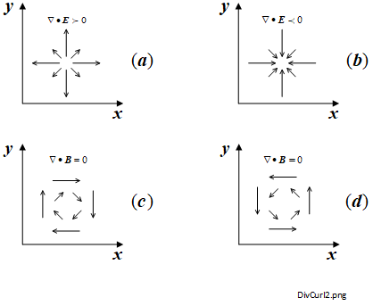
In (a) and (b) the divergence result is always of finite magnitude but is never zero. It shows how the point behaves either as a 'source' or 'sink', in this case of charge which produces or absorbs an electric flux \(\boldsymbol{E}.\) We have adopted the usual convention to consider a source as positive and a sink as negative. (c) and (d) show the result of having a divergence result of zero for a magnetic flux \(\boldsymbol{B}\). The magnetic fields form loops either in a clockwise or counter-clockwise direction depending on the direction of the current.

Curl Operator

The curl operator uses the 'nabla-cross' symbol (\(\nabla \, \times\)), or just the abbreviation 'curl', so the curl of \(\boldsymbol{A}\) could be represented as \(\nabla \boldsymbol{ \times A}\). Similiarly to divergence, it is always applied to a vector. However, in this case the result is another vector. The definition of \(\nabla \times \boldsymbol{A}\) is shown in (1.6-1) in the form of a determinant [3] [4] [5].

\[ \nabla \times \boldsymbol{A} = \begin{vmatrix} \ \hat{\boldsymbol{x}} & \hat{\boldsymbol{y}} & \hat{\boldsymbol{z}}\\[0.8em] \dfrac{\partial}{\partial x} & \dfrac{\partial}{\partial y} & \dfrac{\partial}{\partial z} \\[0.8em] \ A_x & A_y & A_z \\[0.8em] \end{vmatrix} \]

The curl operator was so named because it determines the amount of 'curl' of a vector field and is therefore 'the inverse' of divergence which we discussed in Section 1.5. In Section 1.8 we shall see that the divergence of a curl is zero.

The Divergence Theorem

The Divergence Theorem relates the flux of a vector field passing through a closed surface to the divergence of the field in the volume enclosed. This is shown mathematically in (1.7-1) for a generic vector field \(\boldsymbol{F}\). [1] [3] [4] [5] [6] [7]

\[ \int_{V} \left( \nabla \bullet \boldsymbol{F} \right) \, d V = \oint_{S} \left(\boldsymbol{F} \bullet \boldsymbol{\hat{n}} \right) d S \]

Refer also to Figure 1.9-1. The integral on the left hand side is described by \(V\) for a volume with a smooth surface and no holes. The closed loop integral on the right side, described by \(S\), refers to a surface enclosed by the loop. The surfaces defined for the integration process, similar to those used for Stokes Theorem, are described in Section 1.9. \(d V\) and \(d S\) refer to the elementary small volume and the associated small surface area respectively as the size of both tend toward zero, eventually reaching a point \(\boldsymbol{P}\) on the surface. In the example shown, \(\boldsymbol{P}\) is on a concave surface and the normal unit vector \(\boldsymbol{\hat{n}}\) points outwards. Alternative conventions may be used.

The Divergence of a Curl is Zero

We have the definitions for divergence of a vector in (1.5-1) and for the curl of a vector in (1.6-1). The result of a curl is another vector, therefore the divergence may be taken of this result to give a scalar value. What is that value? The application of these vector operators together with the properties of associativity, which apply to partial differential equations, is shown in (1.8-1).

\[ \begin{align} \nabla \bullet (\nabla \times \boldsymbol{A}) &= \nabla \bullet \begin{vmatrix} \ \hat{\boldsymbol{x}} & \hat{\boldsymbol{y}} & \hat{\boldsymbol{z}}\\[0.8em] \dfrac{\partial}{\partial x} & \dfrac{\partial}{\partial y} & \dfrac{\partial}{\partial z} \\[0.8em] \ A_x & A_y & A_z \\[0.8em] \end{vmatrix} \\ &= \frac{\partial }{\partial x} {\left(\frac{\partial A_z}{\partial y} - \frac{\partial A_y}{\partial z}\right)} - \frac{\partial }{\partial y} {\left(\frac{\partial A_z}{\partial x} - \frac{\partial A_x}{\partial z}\right)} + \frac{\partial }{\partial z} {\left(\frac{\partial A_y}{\partial x} - \frac{\partial A_x}{\partial y}\right)} \\ &= \frac{\partial A_z}{\partial x \partial y} - \frac{\partial A_y}{\partial x \partial z} - \frac{\partial A_z}{\partial y \partial x} + \frac{\partial A_x}{\partial y \partial z} + \frac{\partial A_y}{\partial z \partial x} - \frac{\partial A_x}{\partial z \partial y} \\ &= 0 \end{align} \]

So the result is indeed zero [1] [7].

Stokes Theorem

Stokes Theorem (1.9-1) is a vector identity frequently used in electromagnetics [1] [3] [5] [7].

\[ \int _{S}\left( \nabla \times \boldsymbol{F} \right)\, \bullet d \boldsymbol{S} = \oint_{C} \boldsymbol{F} \bullet d \boldsymbol{l} \]

\(\boldsymbol{F}\), \(\boldsymbol{S}\) and \(\boldsymbol{l}\) the vector arguments of the curl, dot and differential (\(d\)) operators so they are in bold fonts. The operator symbols themselves, \(\nabla \times \), \(\bullet\) and \(d\), are in normal font.

To understand how Stokes Theorem is used, refer to Figure 1.9-1 which shows an arbitrary smooth closed surface \(S\) within the vector field \(\boldsymbol{F}\), in this case using rectangular (\(x\), \(y\), \(z\)) co-ordinates, but of course any 3 dimensional spatial co-ordinate system could be used. A closed loop contour \(C\) in the surface \(S\) is shown, enclosing a small area \(d S\) (in normal font). In this example, \(d S\) is convex but, on some parts of the surface, it could have been concave.

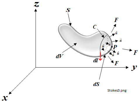
In the limit of integration \(d S\) reduces to a surface with zero volume and zero surface area, in other words a point \(P\). Just before this, over \(d S\) there will be an infinite number of normal unit vectors \(\boldsymbol{\hat{n}}\), a few of which are shown. Here, we are using the convention that the normal unit vector points outwards from a convex surface. As \(d S\) reduces to a point, the normal vector will become normal to the tangential plane at \(P\). This is shown in Figure 1.9-2.

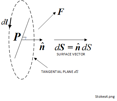
This also shows the arbitrary component of the vector field, \(\boldsymbol{F}\) at point \(\boldsymbol{P}\). \(\boldsymbol{\hat{n}}\) is the unit normal vector to the tangential plane. \(\boldsymbol{F}\) is the component of the vector field at the same point, which could be at any angle. \(d \boldsymbol{l}\) is the tangential elementary vector length within the contour loop at \(\boldsymbol{P}\), now within the tangential plane. At this position, the tangential plane and the normal vector combine to become an orientated area or vector area (\(d \boldsymbol{S}\)) as used on the left hand side of (1.9-1). The vector area \(d \boldsymbol{S}\) is the product of the normal unit vector \(\boldsymbol{\hat{n}}\) and the elementary (scalar) surface area \(d S\).

\[ d \boldsymbol{S} \, = \, \boldsymbol{\hat{n}} \, d S \]

References

1. Pozar, David M.; Microwave Engineering, Third Edition; Wiley International Edition; John Wiley & Sons Inc.; Appendix B, pp 682-683: B1 (Dot Product), B2 (Cross Product), B12 (Divergence of a Curl = 0), B15 (Divergence Theorem), B16 (Stokes Theorem); ISBN 0-471-44878-8.
2. Pozar, David M. (op. cit.); Maxwell's Equations, applications of vector operators; pp 5-9.
3. Kreyszig, Erwin; Advanced Rngineering Mathematics, Fourth Edition; John Wiley & Sons, New York; pp 262-266 (Dot Product), pp 401-404 (Divergence of a Vector Field), pp 406-407 (Curl of a Vector Field and Right-Hand Rule), pp 444-448 (Divergence Theorem of Gauss), pp 454-457 (Stokes Theorem).
4. Kraus and Carver; Electromagnetics - Second Edition, International Student Edition; McGraw-Hill; pp 98-99 (Divergence Theorem), pp 93-97 (divergence of surface charge density), pp 98-99 (Divergence Theorem), pp 175-182 (Curl), pp 34-36 (Gradient); ISBN 0-07-035396-4.
5. Hayt, William H.; Engineering Electromagnetics, Fourth Edition; McGraw-Hill; pp 80-83 (Divergence Theorem), pp 75-78 (divergence definition), pp 254-261 (Curl), pp 106-112 (Gradient), pp 262-267 (Stokes' Theorem); ISBN 0-07-027395-2.
6. Ramo S., Whinnery J. R., Van Duzer, T.; Fields and Waves in Communication Electronics; John Wiley & Sons; pp 76-78 (Dot Product); pp 106-108 (Cross Product); p 85 (Divergence Theorem).
7. Griffiths, David J.; Introduction to Electrodynamics, Fourth Edition; Pearson Education Inc.; pp 2-3 (Dot Product), pp 3-4 (Cross Product); pp 34-36 (Stokes Theorem), pp 31-34 (Divergence Theorem), p 23, 24, 53, 243, 279 (Divergence of a curl is zero). ISBN 978-0-321-85656-2.