Noise Figure and Signal to Noise Ratio
****************************************************************************************************
Electrical noise (noise) in communication and radar systems can be divided into two groups: intrinsic (internal to the hardware) and extrinsic (external to the hardware). In each case 'the hardware' refers to the susbsystem under consideration, such as an amplifier, receiver, filter, or a cascade of 2-port devices. Noise affects all electronic equipment but, depending on its application, some types of noise may be insignificant and others may be critical. In new designs a proper assessment of all forms of noise is required.
Some forms of intrinsic and extrinsic noise are described in the following paragraphs [1] [5] [15].
Additive White Gaussian Noise (AWGN), also known as Johnson, Nyquist or thermal noise, is present in all electrical equipment operating at above absolute zero temperature, or quite simply everything. This is significant in receiving systems, especially through the input stages where the signal strengths are weakest. AWGN is the subject of this article but some other forms of noise will be mentioned for comparison.
Shot noise is caused by the random movement of charge carriers in a solid state device [1].
Flicker noise or \(1/f\) noise occurs in solid state components. Its noise power density varies as the inverse of frequency such as at the output of a mixer close to the beat frequency of of two CW sources [1].
Quantization Noise is generated at the point in a circuit at which an analog signal is sampled to generate a digital signal, such as an analog to digital converter (ADC). It results from imperfect 'rounding' of the instantaneous analog voltage to its digital representation. It manifests in the digital domain as increased bit error rate.
Non linear distortion causes harmonics and intermodulation products when one or more continuous wave signals are present in a device. These products can interfere with wanted signals. This is a common source of noise in real devices which is why we have assumed a linear system for the AWGN analyses.
Radiated susceptibility is one of the properties specified for Electromagnetic Compatibility. The radiated susceptibility of a piece of electronic hardware measures how sensitive it is to noise interference received via the radiative path (electromagnetic waves through 'the air' or free space). The source of this type of noise is usually unintentional but it may be intentional from an adversary to deny service from the hardware. This may be due to imperfect screening, filtering or combinations of both and it may also be a function of conducted susceptibility in mechanisms such as re-radiation.
Conducted susceptibility is one of the properties specified for Electromagnetic Compatibility. The conducted susceptibility of a piece of electronic hardware measures how sensitive it is to noise interference received via the conductive path (through conductors such as cables and metal chassis components). This may be due to imperfect filtering and it may also be a function of radiated susceptibility in mechanisms such as re-radiation.
A plasma is an ionised gas such as lightning or the breakdown which may occur at electrical contacts carrying high powers such as high voltage switchgear. These sources cause electrical noise, both radiated and conducted which may cause interference. This may also be associated with impulse noise
Impulse noise refers specifically to pulse type voltage-time waveforms which contain rapidly rising or falling edges. These include high frequency components which may radiate and/or conduct through cables to the victim hardware. This may also be associated with plasma Noise.
Thermal, Nyquist, Johnson or 'kTB' noise, generically known as additive white Gaussian noise (AWGN) is the type associated with noise factor and noise figure definitions and therefore signal to noise ratio performance. It is generated by all electrical equipment because it is present at temperatures above Absolute Zero. Its mean power is a function of the absolute temperature of the noise source and the effective noise bandwidth of the electrical equipment which generates it [4] [5] [7] [8] [10] [11] [12].
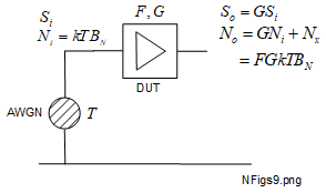
The schematic in Figure 1.3-1 shows how AWGN noise power may be measured for an AWGN source operating at an absolute temperature of \(T\) kelvin (\(K\)).
All components are assumed to be in thermal equilibrium at temperature \(T \,K \) and well matched. AWGN is observed up to frequencies well beyond 100 \(GHz\) so it is present in all electrical equipment operating within the limits of the current technology [7] [13]. The components are assumed to be operating within this range. The AWGN mean power (\(P_n\)) watts (\(W\)) is the product of Boltzmann's constant (\(k = 1.38 \times 10^{-23} J/K\)), the absolute temperature \(T\) \(K\) and the equivalent noise bandwidth of the bandpass filter, \(B_N\) hertz (\(Hz\)). The bandpass filter represents the practical operating bandwidth of the electrical device under test (DUT). In most cases the DUT will be a common 2-port device carrying signals such as an amplifier, attenuator, filter or mixer. If the frequency range has a bandwidth \(B_N\) \(Hz\), then \(P_n\) is given by (1.3-1).
There are many types of electrical noise. In this article we are only considering AWGN, arguably the most important noise affecting the sensitive front ends of receiving systems.
Device scalar gains and losses may be either expressed as logarithmic units (decibels, \(dB\), positive or negative signs) or in linear form (with no units, a positive unit-less real value). The word 'scalar' is emphasised to distuinguish them from vector (phasor) values, expressed in amplitude and phase, which are not applicable here because AWGN amplitude and phase are random. We will adopt the convention of using lower case symbols for logarithmic values and upper case symbols for linear values. Most of the AWGN related equations are less cumbersome to manipulate with linear units but many datasheets and test equipment measurements use logarithmic units. In this article for brefity we may sometimes omit the adjective 'logarithmic' but we will always use the correct units, if any. Therefore, whenever values are defined in \(d B\) they are logarithmic, otherwise they are linear.
The general expressions for gains and losses are provided by the equations in (2-1), (2-2) and (2-3)
Note that some of the symbol definitions provided in the references are inconsistent. Here we will define noise figure (lower case 'f', \(f\)) as the logarithmic value and noise factor (upper case 'f', \(F\)) as the equivalent linear value. Therefore, these are related by (2-4):
Signal to noise ratio (\(S N R\)) is the signal power \(S\) watts divided by the AWGN power \(N\) watts. In order to carry information the signal occupies a finite bandwidth to accommodate some form of modulation. This, plus suitable margins or guard bands typically defines the noise bandwidth that the DUT is designed for. The noise bandwidth determines the AWGN power \(N\). Real 2-port devices can only degrade the \(S N R\) at the DUT output relative to the input, by adding AWGN originating in the device itself. In many cases the continuous wave (CW) waveform gain, measured for example using a vector network analyzer (VNA), is used as the signal gain. This must be used with caution because CW is very narrow band but AWGN is potentially broadband. The noise factor \(F\) of the device is a measure of how severely the \(SNR\) is degraded by the device from the input to the output. For the DUT input and output SNR definitions we simply add the subscript \(i\) or \(o\) to the sybol as required, (2-5) and (2-6).
Each of the stages within a cascade has a (linear) noise factor \(F_n\) and linear gain \(G_n\), where \(n\) is the number of the stage, the first stage in the direction of the signal by convention being '1'. We will proceed to investigate the noise, gain and \(SNR\) performance of cascaded stages like these. The conditions assumed are listed in the following paragraphs.
The stages typically have symmetric input and output impedances compatable with common test equipment, such as 50 \(\Omega\) unbalanced (coaxial), but this is not essential. Whatever impedances are used, they must all be well matched to minimise reflections. Scalar match performance is commonly measured using return loss or VSWR across the operating frequency range plus suitable margins.
When considering a cascade of 2-port devices, at the output, immediately before the detector, there must be a bandpass filter with a defined center frequency and noise bandwidth. This would be specified to filter out the maximum bandwidth of the signal spectrum (the CW carrier plus modulation) and reject adjacent channel noise. This must be specified appropriate to the modulation and channelisation schemes used by the DUT in normal operation. Its transmission frequency response should be positioned within the aggregrate operating bandwidths of all earlier stages and would therefore determine the AWGN contribution to the \(SNR\) performance for the whole cascade.
Many types of noise are seen in communication and radar systems but here we are only considering Additive White Gaussian Noise (AWGN). AWGN is also known as thermal, Johnson or Nyquist noise and is derived from black body radiation [1] [14] [15] [16]. Other types of noise will require alternative analyses.
For the AWGN related theory, a noise-free sinusoidal continuous wave (CW) waveform of defined frequency and amplitude is assumed to represent the signal. The AWGN noise itself is assumed to come from a calibrated AWGN source operating at a specified equivalent absolute temperature. Of course, the performances of real CW and AWGN sources fall short of theoretical (ideal) ones and these inadequacies must be allowed for in real designs.
It is assumed that the operating signal and noise levels cause negligible component heating and the stages (devices) run at very high efficiency (there is negligible internal heating). Also they must have been allowed to thermally stabilize at the defined ambient temperature before any measurements. Usually, our interest in noise figure is greatest at the front end of the receiver stages where the incoming signal is expected to be small anyway. Note that the measured noise factor of a device does change with the input AWGN spectral power density as well as with the temperature of the device itself. Ambient operating temperatures must be measured accurately. Therefore, noise figure measurements are commonly standardized in datasheets to 290 \(K\), the standard noise temperature \(T_0\) or approximately (27 \(^\circ C\)). In the early days of radio-astronomy this temperature was chosen as an 'average' room temperature across the world. In hotter and cooler room environments, informal measurements within a few degrees of \(T_0\) are often acceptable after allowing for temperature stabilisation. For operating in non-room environments, for example in space or when force-cooled, corrections may be applied.
False. I would argue that it now has even more relevance than ever before in modern cable and wireless systems. Just a few examples are digital cellular (3G, 4G, 5G, 6G), Wi-Fi based (IEEE 802.11), WiMax based (IEEE 802.16), digital terrestrial broadcasting, deep space communications, broadband cable (DOCSIS), primary and secondary radar receivers. All of these require to exploit the lowest possible device noise factor to minimise the degradation of signal to noise ratio on the receive side. This reduces the necessary transmit powers, similarly reducing the transmitter design, production, installation and running costs. As the radio spectrum is shared, and wireless service areas generally overlap in a planned way to avoid coverage breaks and allow the handover protocol. All communication services require transmit powers to be minimised to reduce interference to other users and to maximise the overall capacity available. Reduced noise factors of the receive equipment therefore ultimately leads to increased capacity overall.
We have made many references to additive white Gaussian noise (AWGN) so some more background information on the physics behind this is included in the following sections.
For a resistor \(R\) ohms (\(\Omega\)) at an absolute temperature \(T \) kelvin (\(K\)), the random and independent motion of large numbers of electron charges results in voltage fluctuations across the resistor with a Gaussian distribution. The average vector voltage of the AWGN is zero, but the mean square voltage is finite and proportional to the mean power of the AWGN for a given bandwidth. The root mean square (RMS) value of the noise voltage, \(V_n\) volts (\(V\)), is given by Planck's black body radiation law, (3-1) [1] [7] [9].
where:
The instantaneous noise voltage within a defined noise bandwidth is not coherent or sinusoidal, its resultant vector or phasor voltage being zero, but the mean square voltage is finite and proportional to the mean AWGN power. The adjective 'additive' in the AWGN acronym describes how the noise powers of contiguous frequency bands may be simply added to yield the noise power of the aggregate band. This is a very useful property of AWGN. We will first apply this equation exactly and then simplify it to derive the \(k \,T B\) form.
With an average (vector) value of zero, we cannot extract a phasor value from (3-1). However, the associated noise power is finite and proportional to the mean square voltage. To calculate the AWGN power, we need to incorporate the noisy resistor \(R\) into a perfectly matched Thevenin equivalent constant voltage circuit as shown in Figure 3-1. This includes a noise-free source resistor also of resistance \(R\) and an ideal 'brickwall' bandpass filter (BPF). We will see that the 'white' property of AWGN extends to beyond 100 \(GHz\) so the BPF is required to restrict the noise bandwidth under consideration (\(B_N\)) to some useful range relevant to the 2-port devices in use [7] [13].
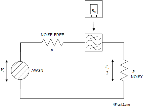
Figure 3-1 shows that, to calculate the mean AWGN power (\(P_n\)) we must use, not \(V_n\) but \(V_n/2\) (3-2):
We have also substituted for \(V_n\) from (3-1). Popular units for describing AWGN power spectral density, say \(PSD1\), is decibels relative to one milliwatt per hertz (\(dBm/Hz\)). \(P_n\) (in watts) must initially be multiplied by \(10^3\) to convert to milliwatts, then divided by \(B_N = 1 \, Hz\). Then, ten times the logarithm to base 10 of this value gives the result in these units (3-3).
We are using \(T=T_0\) again for which \(PSD1\) is the red plot in Figure 3-2

The \(PSD1\) plot shows the AWGN noise power density to be constant at about -174 \(d B m/Hz\) up to about 1000 \(G H z\) after which it tails off steeply. However, the current generation of electronics hardware based on conductors (circuit and waveguide technology) is included within this frequency range and the tail-off should not concern us too much. The flat region of \(PSD1\) demonstrates the 'white' property of AWGN, the analogy being with the optical part of the electromagnetic spectrum and its component colours.
Now we will make a very useful simplification to obtain the less cumbersome \(k T B\) form of equation derived from (3-2). For frequencies below about 100 \(GHz\) and at operating temperatures close to 'room temperature', approximately \(T = 290 \, K\), \(h f \, \lt \lt k T \) is valid and the first 2 terms of a Taylor series gives (3-4) [1]:
Using (3-4) in (3-1) results in (3-5), also known as the Raleigh-Jeans approximation [1].
This equation is sufficiently accurate to use for all electronic equipment at the current limits of the technology. For very low temperatures and/or very high frequencies, using (3-1) directly may be slightly more accurate. The same procedure applied for the 'exact' equation using the Thevenin equivalent circuit shown in Figure 3-1 may then be applied to arrive at the well known AWGN equation (3-6).
We know that \(k = 1.38 \times 10^{-23} \, J/K\) is Boltzmann's constant. \(T\) is the absolute temperature of the AWGN source. I have added the subscript '\(N\)' to the bandwidth symbol '\(B\)' to emphasise that it refers to the (AWGN) noise bandwidth as opposed to say, the -3 \(dB\) CW (VNA-based) bandwidth, or to some other definition of bandwidth [9] [15]. The noise bandwidth of a real bandpass filter is the bandwidth of the equivalent rectangular ('brickwall') response shape as it affects AWGN. For most cases, the relevant noise bandwidth is that which affects the whole cascade of 2-port devices from the signal input to immediately before the detector. This is examined further in Section 3.2. An important and useful property of this equation is that it is not a function of the absolute frequency, but it is a function of noise bandwidth itself. The AWGN may be expressed as a noise power density (NPD) with respect to frequency or spectral power density (SPD) by dividing (3-6) by \(B_N\) (3-7).
After again converting this to units of \(dBm/Hz\), it is included as \(PSD\,2\), the blue plot in Figure 3-2. Comparing the red and blue plots shows that the simpler version of the AWGN equation, (3-6), is adequate for frequencies up to around 1000 \(GHz\). Therefore, a common condition of using (3-6) is that the absolute frequency must be less than about 100 \(GHz\).
The next question is usually, "What noise bandwidth should I actually choose for a particular system?". This decision needs to consider the devices under test and the objectives against the limitations of the test equipment. These will be discussed in Section Section 3.2
A 2-port device under test (DUT) has both an operating bandwith and an equivalent noise bandwidth, or simply 'noise bandwidth' \(B_N\). We also need to know its various other properties such as input and output operating frequency ranges, its channelisation scheme and modulation characteristics. Noise bandwidth should be used in any analyses which relate to AWGN.
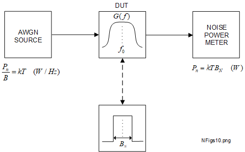
The operating bandwidth of a DUT is usually measured using a continuous wave (CW) frequency source, typically part of a correctly set up and calibrated vector network analyzer (VNA). VNA measurements may be repeated across a range of stepped CW frequencies, usually selected to extend slightly beyond the expected operating bandwidth. The noise bandwidth of the DUT may be measured empirically using a broadband AWGN source connected to the DUT input and a sensitive power meter connected to the output. This is shown in Figure 3.2-1.
The equivalent noise temperature used for the AWGN source (\(T \, \, K\)) and the power meter sensitivity must be chosen appropriately for the DUT bandwidth. Achieving this is sometimes challenging. Alternatively, the noise bandwidth may be calculated if accurate DUT transmission data are known. Most modern, high specification VNAs enable us to export this electronically into 'number crunching' applications for further processing such as Excel® and Matlab®.
As we mentioned, the noise bandwidth of a DUT is the bandwidth of the equivalent rectangular (or 'brickwall') passband filter, referenced to the same transmission amplitude and center frequency, that will transmit the equivalent mean AWGN power if it replaced the DUT. This may be shown using the normalized example transmission responses in Figure 3.2-2 represented by the blue and red continuous plots. This demonstrates how two different devices may have the same VNA (CW-based, -3 \(dB\)) bandwidths but differing noise bandwidths.

A noise bandwidth may be calculated for any DUT transmission response but those with near symmetry about a center frequency, like either of those shown in Figure 3.2-2, are typical. In this example, the center frequency is 100 \(MHz\) coincident with the minimum insertion loss. Here, the response is normalized so this corresponds to a magnitude of one. This frequency will be used as a reference for the actual response and the noise bandwidth response.
Referring to Figure 3.2-1, if the effective noise temperature of the AWGN source is \(T = T_0 = 290 K \), the noise power spectral density (NPD) from it, feeding the DUT, is \(k \,T_0 \,\, \,W/Hz \). The total mean noise power passing through the DUT \(P_T\) is given by (3.2-1), where \(G(f)\) is the function describing the linear scalar transmission of the DUT with respect to frequency. This is equivalent to the area under the response plot.
A practical upper integration limit of 100 \(GHz\) was chosen based on the Rayleigh-Jeans criteria from Planck's black body radiation law, giving a relatively flat AWGN NPD. This was discussed in Section 3.1 and allows us to use the simplified AWGN equation (3-6). After substituting the real DUT for the hypothetical noise bandwidth (\(B_N\)) filter, noting that the transmission amplitude is now referenced to its value at the center frequency of the real DUT, \(G(f_0)\), \(P_T\), again the area under the response is (3.2-2).
Normalized responses, say \(G_N(f)\), of the type shown in Figure 3.2-2 are defined as (3.2-3).
By equating (3.2-1) with (3.2-2), and using the definition in (3.2-3) gives the following expression for \(B_N\) (3.2-4).
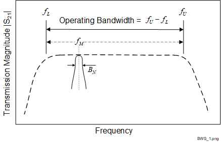
The example DUTs shown in Figure 3.2-2 have -3 \(dB\) bandwidths of about 5 \(MHz\) and we suggested that these may have been measured using a VNA. In order to perform AWGN measurements on these to a similar frequency resolution, such as those necessary for noise figure, the noise figure meter (NFM) would need to step a narrow measurement noise bandwidth \(B_N\) transmission response across the operating band in small increments. Suppose the operating bandwidth extends from a lower frequency \(f_L\) to an upper frequency \(f_U\), plus a suitable margin, then we would require (3.2-5).
So, for an operating bandwidth of around 5 \(MHz\) we might expect the \(B_N\) of the NFM to be perhaps a few tens of kilohertz. If you have the budget, this can be done with some of the latest noise figure analyzer (NFA) test equipment [20]. In fairness to the NFA manufacturers, I would add that the latest NFAs generally have DSP-based, real-time architectures, numerous add-on options such as spectrum analysis and resolution bandwidths down to 1 \(Hz\). Otherwise, we will be using the Hewlett Packard (HP) Noise Figure Meter (NFM) model HP 8970B with the switched AWGN 14 \(dB\) ENR noise source HP 346B [16]. These instruments may be considered 'legacy' but they were widely respected industry standards for many years. The HP 8970B has an input frequency range from 10 \(MHz\) to 1600 \(MHz\) with a bandwidth of 'approximately 4 \(MHz\)'. This approximates to a noise bandwidth also of 4 \(MHz\), with a center frequency tunable across the input frequency range. For now we are assuming the DUT is a device without internal frequency conversion, such as an amplifier, attenuator or filter. Also, the DUT operating frequency range is within the frequency ranges of both the NFM and the noise source (we are not including any frequency conversion external to the DUT). DUT measurements with frequency conversion will be addressed in Section 5.5. Figure 3.2-3 shows how the noise bandwidth \(B_N\) of the NFM may be swept across the operating bandwidth of the DUT \(f_U - f_L\) for a typical noise figure measurement.
Noise power spectral density (PSD) or simply noise power density (NPD) are alternative descriptions of the same property, the AWGN power density with respect to (absolute) frequency. As discussed in Section 3.1, as long as the operating frequency is less than about 100 \(GHz\) and temperature stable, a calibrated AWGN source will generate a constant NPD which is not a function of frequency [7] [13]. Most practical receiving systems operating with today's technology will have operating bandwidths which are much less than 100 \(GHz\). The majority of traffic channel bandwidths in communications and radar have evolved to a range from about 1 \(MHz\) to 100 \(MHz\). With careful frequency planning, the operating bandwidth of a DUT such as a low noise amplifier (LNA) can be designed to cover several such traffic channels. The same product can potentially be selected by several customers such as telecommunications service providers, each with slightly different traffic allocations.
The Y-factor method, described in Section 5.4, is often used by NFMs and NFAs for accurate and quick noise figure and noise gain measurements. This also requires a 'noise source' such as the HP 346B. The HP 346B and other similar devices, actually comprises two AWGN sources, each with accurately known noise temperatures and controlled by the associated NFM or NFA. The 'white' adjective in the AWGN acronym, being an analogy with white light in the optical spectrum, means that the AWGN power density across the operating frequency range is nominally constant. Actually, due to practical design limitations there is usually some small variation with frequency but this can be corrected for during calibration.
A popular unit for AWGN NPD is the logarithmic: 'decibels relative to one milliwatt per hertz', with the symbol \(dBm / Hz\). This does not imply that literally measuring the AWGN in a 1 \(Hz\) bandwidth is necessary (although it is possible with some of the latest high specification NFAs) [20]. Substituting the standard noise temperature of \(T = T_0 = 290 K\) and noise bandwidth \(B_N = 1 Hz\) into the AWGN power equation (3-6) tells us that the AWGN power in 1 \(Hz\) is -174 \(dBm\). This is difficult to measure directly, but the white property of AWGN here is useful and this is one example of its use. Widely available and relatively inexpensive noise figure equipment will typically have measurement (noise) bandwidths in the order of a few megahertz. The white property of AWGN means that the noise power measured in, say a 4 \(M H z\) noise bandwidth, may simply be linearly scaled down to narrower bandwidths such as 1 \(H z\) to convert it to the \(dBm / Hz\) unit. This example would be a linear factor of \(0.25 \times 10^{-6}\) or a logarithmic value of \(10\log_{10}(0.25\times 10^{-6}) \, dB\) or \(-66 \, dB\). To obtain such a value accurately would require the larger noise bandwidth to be known precisely.
In many of the references there is some inconsistency in the use of the terms noise factor (\(F\)) and noise figure (\(f\)). As described in Section 2 under 'Linear and Logarithmic Units', we will keep with the convention of \(F\) being the linear form, expressed as a unitless positive real number greater than or equal to 1, and \(f\) being the logarithmic form, expressed as a positive value in \(dB\).
Noise factor will be described with the help of the schematic showing the 2-port device under test (DUT), which does not have frequency conversion, with the test equipment shown in Figure 4.1-1.

It is assumed that the DUT is well matched at both ports to the test equipment and all devices are in thermal equilibrium. The ambient temperature of the DUT should be controlled and stabilized to the standard noise temperature, \(T_0 = 290 K\). The dotted box contains a sensitive, RMS sampling power meter and a bandpass filter with a tunable center frequency to represent a simplified noise figure meter (NFM). The AWGN source is broadband, selected to cover a frequency range in excess of the operating bandwidth of the DUT. The frequency range of the NFM \(f_M\) must be within the operating frequency range of the AWGN source and cover the operating frequency range of the DUT, \(f_L\) to \(f_U\). The noise bandwidth \(B_N\) for all measurements is defined by the tuneable bandwidth of the NFM. For the best frequency resolution, \(B_N\) must be much less than the DUT operational bandwidth as was described in Section 3.2. Although this configuration does not use a CW source signal similar to a VNA, under the conditions described it may use the AWGN source to measure gain. For calibration purposes, the DUT may be removed and the combined sources connected directly to the NFM including any cables and adaptors necessary for the measurement. For measurements, the DUT is inserted as shown. The calibration and measurement configurations allow both linear gain of the DUT (\(G\)) and its noise factor (\(F\)) to be measured. Under these conditions, \(G\) is equivalent to the linear gain that could be measured using CW with a VNA.
The DUT input CW (signal) power is \(S_i\) and the input AWGN power is \(N_i\). The DUT output CW power is \(S_o\) and the output AWGN power is \(N_o\). All powers are linear, specified in watts (\(W\)).
The noise factor definition for a matched 2-port device like this DUT is the ratio of the signal to noise ratio (SNR) at the input divided by the SNR at the output. The linear gain is \(G = S_o / S_i\) and \(N_i\) equates to \(P_n\) in (3-6). \(F\) is therefore expressed by the following equation (4.1-1).
\(B_N\) is not the noise bandwidth of the DUT alone, which would be a value similar to its operating bandwidth, but a much smaller value chosen according to (3.2-5). As \(F\) is a function of \(T\), the latter must be specified and appropriate to the system under consideration. Linear (small signal) conditions are assumed. Therefore the DUT gain has an equivalent effect on both signals and noise. Here we have assumed the ambient temperature of the source and DUT to be the standard noise temperature as is frequently used in datasheets, \(T = T_0 = 290 \, K\). For antenna receive systems or unusually hot or cold environments, the actual noise factor will change accordingly.
For AWGN related parameters (noise factor, gain and SNR), 2-port devices may be represented schematically like the example shown in Figure 4.1-2.
Not to be confused with similar schematics for the Thevenin and Norton equivalent circuits, this AWGN schematic displays the real DUT input and output mean noise powers, and how they relate to each other. AWGN phase is random and therfore unpredictable. Power has a square law function of instantaneous voltage so does not have a phase. Therefore we can only use mean power levels or mean square voltages to describe AWGN levels. These are real powers so they are additive, hence the first letter of the AWGN acronym. Within a cascade, the stages are assumed to be well matched so there are no issues with standing waves or reflected power. In fact there are no 'waves' as nothing is sinusoidal and there is no phase reference as would be provided by a sinusoidal source. That is why we have given the symbol for the AWGN source a hatched appearance.
From (4.1-1) \(F\) is a function of \(N_i\). With the AWGN source, we know from (3-6) (\(N_i = P_n\)) that \(F\) is also a function of the effective noise temperature of the AWGN source \(T\). This shows an important property of the noise factor definition. The noise factor is actually dependent on the NPD (3-7) from the source, feeding the DUT input. In datasheets, the effective temperature of the AWGN source is often standardised to 290 \(K\). This is an evolution of 'average' room temperature adopted for convenience in the design of low noise amplifiers in the early years of satellite communications and radio astronomy. It is now an Institution of Electrical and Electronics Engineers (IEEE) accredited definition [19]. It assumes that the equivalent input noise temperature (\(T_0\)) is 290 \(K\) which, using the discussion in Section 3.1 and (3-7) gives a NPD of -174 \(dBm/Hz\). There was clearly an assumption that, in most cases, the low noise device under consideration was operating at approximately room temperature.
Take the example of a narrow beam receiving antenna, typical of the type used for satellite communications [27]. This is highly directional and designed to only collect emissions from a small near circular aperture in space when pointing at the position of the satellite. We will assume it is an ideal antenna with zero loss and perfectly matched to the first stage of the receive cascade, a low noise amplifier (LNA). If the satellite transmitter was 'switched off' the ground antenna would then collect sky noise source(s), which approximate to AWGN, from the same direction as the satellite. With the exception of possible periods of Sun interference, the only AWGN sources are from distant stars. Distances from these are huge, usually measured in light-years. Furthermore, the AWGN power flux density (PFD) of noise from a distant star will suffer 'spreading' to an inverse square law towards the Earth [24] [25]. The linear SI unit for PFD is watts per square meter (\(W/m^2\)). The combined PFDs of noise sources like these from many stars arriving at the Earth have been measured accurately. Some such measurements arrived at an equivalent antenna noise temperature sometimes below 50 \(K\) [23]. If we had tested the LNA designed for this antenna in the laboratory, assuming the standard noise temperature of \(T = T_0 = 290 \, K\), the SNR after implementation would actually be greater. Therefore, when designing low noise receiving systems like these, we have to make the necessary corrections. In Section 6 we will look at a similar example.
Antennas used for terrestrial communications tend to have noise temperatures closer to 290 \(K\) because the beam shapes typically include substantial natural ground sources which are much closer to this temperatue than, say 50 \(K\). Also, they are physically much closer, so the beam spreading due to the inverse square law is less significant. However, assuming that noise from the Sun is not within any part of the beam, this is offset by the upper part of the beam which will usually see sources at colder temperatures.
Figure 4.1-2 shows a schematic for a 2-port 'noisy' DUT together with symbols for the parameters which were described in Section 4.1. The adjective 'noisy' simply means that the DUT is a real, imperfect device which adds some finite level of AWGN to the signal applied to the input. The AWGN will only be zero in a device that is at zero degrees absolute (\(0 \, K\)), so all real devices are 'noisy'.
The first task is to choose a measurement or noise bandwidth \(B_N\). We will choose 4 \(MHz\), as we have the HP 8970B NFM in mind as an example. Ideally this should be much less than the operating bandwidth of the DUT but we can live with it being just slightly less provided we are very careful with the choice of the measurement frequency (the center frequency of the tuneable bandpass filter device within the NFM). We need to avoid inadvertantly tuning to the side of the passband response. Examples of modern, high specification noise figure analyzers (NFAs) can have measurement bandwidths as small as 1 \(Hz\) [20]. The 'additive' and 'white' properties of AWGN mean that the AWGN measured in a wide bandwidth like 4 \(MHz\) can be scaled linearly down to a narrower bandwidth. However, this conversion must be performed with caution as the measurement bandwidth transmission characteristic needs to be measured very accurately.
We must also consider the smallest service channel bandwidth carried by the DUT which requires testing. For example, a DUT designed with an operating bandwidth of 500 \(MHz\) targetted at several 4G and 5G digital cellular service providers may be required to carry channel bandwidths as small as 5 \(MHz\). High resolution noise figure (and gain) data would be useful for potential customers to consider.
Using (3-6) with \(N_i = P_n\) and \(T_0 = T\), gives us the noise factor definition (4.4-1).
We are assuming the standard temperature of \(T = T_0 = 290 \, K\) is used for the AWGN source, so essentially a 'room temperature' application. In this noisy DUT the output noise power comprises 2 additive components: the amplified input noise \(G k T_0 B_N\) and the noise added by the DUT itself or 'excess' AWGN, say \(N_x\), referred to the output (4.4-2). \(N_x\) does not depend on either the input signal or noise power, it is only a function of the DUT electronics hardware and the temperature at which it is operating, in this case \(T_0\).
Substituting (4.4-2) into (4.4-1) gives (4.4-3)
As \(N_x\) is an AWGN (output) power, it may be represented as an equivalent temperature using (3-6) in the same noise bandwidth \(B_N\). It is most commonly represented as an equivalent input noise temperature \(T_e\) but could equally be represented as an equivalent output noise temperature. We will chose the former so that the \(GkB_N\) parts cancel out. Therefore, to express \(N_x\) in terms of \(T_e\) we need (4.4-4).
Substituting \(N_x\) from (4.4-4) into (4.4-3) gives us the very important noise factor relationship (4.4-5).
An attenuator, unlike an amplifer, is not connected to a power supply and therefore the source of AWGN is limited. This might sound counter-intuitive because we know that an attenuator comprises a network of accurately trimmed resistors designed to attenuate a signal (or noise) whilst maintaining a good input and output match. Yes, resistors generate noise if they are acting as a source but they also attenuate noise in the same way that they attenuate signals. An attenuator is a 2-port device just like an amplifier and does not behave like a one port AWGN source, for example a noise source or an antenna. To calculate its noise factor, we simply apply the same definitions used for any other 2-port linear device. In fact it is more straightforward than an amplifier: because it is passive, we can call upon conservation of power.
Figure 4.6-1 is a circuit schematic for an attenuator. The example is a 'pi' style unbalanced type, such as a 50 \(\Omega\) coaxial device but it could be any type of correctly matched attenuator, balanced or unbalanced.

The attenuator must be well matched to adjacent stages and in thermal equilibrium at the standard noise temperature \(T_0 = 290 \,\, K\). Before proceeding, we must be familiar with the definitions used for linear and logarithmic gains and losses. These are given in Section 2 under 'Linear and Logarithmic Units'.
The equations will continue to use symbols expressing linear values. An exception is the common attenuator description found in datasheets, or logarithmic loss such as 3 \(dB\). The linear (upper case 'l', unitless) and logarithmic (lower case 'l', dB) values for loss are related by: \(L=10^{l/10}\). For example, a 3 \(dB\) attenuator has a linear loss of 2.0.
Referring to Figure 4.6-1, a noise power of \(N_i \, W\) applied to the input port will be attenuated by linear value \(L\) and then exit the output port. As there is no power supply, by the conservation of energy, the power that was removed to 'create' the attenuation is equivalent to the excess noise power \(N_x\). As we have specified thermally stabilised conditions, we are actually using conservation of power (4.6-1).
The next step is to express the attenuator noise factor \(F\) in terms of excess noise and its loss, very similar to the amplifier case (4.4-3) but here substituting \(G=1/L\) .
Then substituting for \(N_x\) from (4.6-1) into (4.6-2) gives the result for \(F\) (4.6-3).
Converting to logarithmic units which may be more convenient, the loss of an attenuator in \(dB\) is equivalent to its noise figure in \(dB\).
Cascaded 2-port stages are used extensively in communications and radar systems. Their use in receiving systems is of particular interest relating to AWGN because of the desire for low noise. Some reasons for the cascade architecture are listed below.
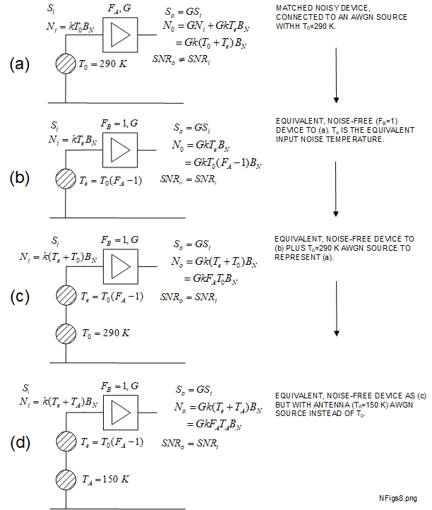
A very useful approach for cascaded AWGN problems is to start with the AWGN schematic as shown in Figure 4.1-2, then convert this to an equivalent which comprises a hypothetical noise-free DUT with a separate AWGN source at the input represented by \(T_e\). The gain of the DUT remains unchanged. This procedure is shown in Figure 5-1 with the help of (4.4-3) and (4.4-5).
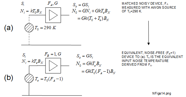
Using the signal and noise equations that were described in Section 4, Figure 5-1(a) shows how a DUT with a noise factor of \(F_A\) and linear gain \(G\) may be represented. Here, the AWGN source connected to the input represents that used for the noise factor measurement using the \(T_0\) = 290 \(K\) standard. This does not contribute in any way to the internal noise of the DUT, other than to how it is defined.
Figure 5-1(b) is equivalent to (a) but with the internal DUT noise expressed by \(T_e\) referred to the input, obtained from (4.4-5). This schematic shows how this noisy device may be included into a cascade. Moving \(T_e\) values to various input and output positions of the DUTs within a cascade simplifies \(SNR\) related calculations.
To investigate how the \(SNR\) is affected using the same DUT used in Figure 5-1 but with sources of different AWGN properties, refer to Figure 5-2.

One advantage of representing the DUT as shown in Figure 5-1 (b) is that its gain is unaffected by any of the noise manipulations. Therefore, the position of \(T_e\) from any device within the cascade may be modified by the appropriate gain factor(s) to other position(s) within a cascade. The derivation of the Friis cascaded stages formula in Section 5.1 demonstrates this principle [3] [13] [19].
Now we will derive Friis's cascaded noise factor equation which is very useful for understanding the small signal noise performance of cascaded stages. Again, the assumptions are that each device is operating linearly and well matched to the next and all devices are in thermal equilibrium at the same temperature as the source, which we will take as being the standard noise temperature of 290 \(K\). This approach applies to an input AWGN also at 290 \(K\), such as a nearby signal generator. If the input is a 'colder' source, such as a satellite antenna, we need to take the equivalent input noise temperature approach, which will be described. Refer to Figure 5.1-1.

Figure 5.1-1(a) shows two cascaded stages: 1 and 2 ordered in the direction of the signal-flow. For each, the noise factor and gain symbols are \(F_n\) and \(G_n\) respectively where \(n\) is the stage number. The schematic symbols for amplifiers are used simply for convenience, the same theory applies equally to any other linear 2-port matched devices: attenuators, filters, couplers etc..
Figure 5.1-1(b) is the result of connecting together stages 1 and 2 with each device represented by an equivalent noise-free (\(F=1\)) DUT with an input noise temperature added of the form \(T_{en}\), calculated from (4.4-5). The gains are unchanged and have identical effects on the signal and noise powers as was described in Section 5 and Figure 5-1. In Figure 5.1-1(c), \(T_{e2}\) has been transferred from the input of stage 2 to the input of stage 1, at the same time correcting the value by the reciprocal of \(G_1\), \(1/G_1\). As the noise temperatures are linear functions of AWGN power, they may simply be added as shown in Figure 5.1-1 from (b) to (d).
Assuming the equivalent device for the two cascaded stages has a total gain and total noise factor of \(G_{2T}\) and \(F_{2T}\) respectively, then \(G_{2T}\) is simply the product of each gain separately (5-1).
Then (4.4-5) is applied to the schematic representing the \(T_{e}\) value for the equivalent total equivalent input temperature \(T_{e2T}\) (5-2).
From Figure 5.1-1(d) the expression for moving the individual stage \(T_e\) values to the input is (5-3)
Then substituting the \(T_{e1}\) and \(T_{e2}\) values from Figure 5.1-1(b), (5-4) and (5-5), into (5-3) gives (5-6).
It will be clear from the procedure described for 2 cascaded stages: \(G_{2T}\) (5-1), \(F_{2T}\) (5-2) and \(T_{e2T}\) (5-3), that these may be simply extended to as many stages as required by a linear progression. For example, for 3 stages using the same symbol conventions, \(F_{3T}\), \(T_{e3T}\) and \(F_{3T}\) are given by (5-7), (5-8) and (5-9).
From (5-6) we can see that \(F_{2T}\), the overall noise factor of the cascade, in this case only 2 stages, is a significant function of the properties of stage 1 (\(F_1\) and \(G_1\)). In order to minimise the degradation of \(SNR\) caused by the cascade, \(F_1\) must be minimized whilst \(G_1\) must be maximized. Most well designed low noise receive systems therefore include a front-end (stage 1) device with a small noise factor and appreciable gain across the operating frequency band.
Taking the cascade a stage further, it is well known and proved in Section 4.6 that the noise figure of a matched attenuator is equivalent to its logarithmic loss. An interesting exercise using (5-9) is to add such an attenuator to the front end of the cascade and confirm that its effect is to increase the total noise figure of the whole cascade by the same amount as the attenuator loss. Also, the total gain of the cascade is reduced by the same amount, therefore causing two contributions to the degradation of \(SNR\). Therefore the temptation of using a long, relatively high loss, feeder cable from a distant receiving antenna to a receiver may seriously degrade performance.
Most receive systems will comprise many stages and groups of contiguous stages may be analyzed successively. This is usually performed starting at stage 1 because (5-3) and (5-6) show that this is the most critical for AWGN performance. Stage 2 and subsequent stages become progressively less critical.
Further to Section 5.1 a common question is: "How do I trade off the gains and noise factors of my proposed front end devices for the best noise performance?" One way is to consider 2 front end candidate stages, such as those shown in Figure 5.1-1(a) with the noise factors (\(F_1\) and \(F_2\)) and gains (\(G_1\) and \(G_2\)) as shown. Now consider that the symbol subscripts refer, not to the stage positions, but to the physical devices: numbers, 1 and 2. Suppose, for the order shown in Figure 5.1-1(a), the overall noise factor for the 2 stages is \(F_{TA}\) and for the reverse order (stage 2 followed by stage 1) it is \(F_{TB}\). Then, by applying (5-6) in both cases results in (5.2-1) and (5.2-2) [13].
If we had assumed \(F_{TA} \lt F_{TB} \), then, using (5.2-1) and (5.2-2) creates the following inequality (5.2-3).
The noise measure (\(M\)) of a 2-port device is defined as [13]:
Comparing the noise measure of each of two candidate 2-port devices may therefore be used to determine which device should be first in the signal path to provide the best overall noise performance.
Antenna (equivalent) noise temperature is less a function of the antenna electrical design and more a function of 'where it is pointing', the 'sharpness' of the main lobe and the degradation caused by unwanted side lobes and back lobes. To examine the causes we need to make some assumptions which are listed below.
We are assuming free space propagation conditions. Usually, these are readily achieved with 'line of sight' satellite and space communications, as opposed to typical terrestrial communications. The free space antenna links must be direct only and free from reflected, refracted or diffracted components. Antenna noise temperature is still an important in terrestrial communications, but this will be addressed after considering the direct path.
especially cellular, reflections and multipath propagation is a fact of life which is to achieve greater capacity with features such as 'multiple in multiple out' (MIMO) antenna configurations. The principle of minimising AWGN is still important here but antenna noise temperature is less important. A typical application where it is critical would be in a satellite downlink where we may exploit the cold sky temperature 'seen' close to the same direction as the satellite.Despite the popularity of near field communication (NFC) devices, most wireless communication including that we are considering, are still designed to operate in the far field, also known as the Fraunhofer region. The far field region is beyond a minimum distance from the transmit or receive antenna which allows us to use a range of accurate and reliable approximations similar to geometric optics. These need to be complied with for both the transmit and receive antennas on the same link simultaneously. There are a few empirical formulas which have been developed to estimate this distance, say \(x_{ff}\) [21], [22], [26]. Perhaps the most common one is (5.3-1).
For all communication systems in which antenna noise temperature is a critical, the link distances will be sufficient that all antennas are working well into their far fields.
A perfect antenna has an efficiency of 100% and its gain function will be identical to its directivity function. This condition will be assumed for all the considered antennas. Practical antennas will have some additional loss elements generated by: imperfect coupling, finite conductivity of the component parts and dielectric loss components. The aggregate 'front end loss', or front end attenuation, heavily affects the AWGN performance of the whole receive chain (cascade) and is considered in Section 4.6.
An antenna is an interface between a transmission line such as a cable and the propragation medium, typically 'the air'. Provided the air is unpolluted and reasonably free from precipitation, it approximates to free-space. The antenna is assumed to be simultaneously matched to the cable impedance, such as 50 \(\Omega\), on the conductor side and to the intrinsic impedance of free space (\(\eta_0\)), approximately 377 \(\Omega\) for plane wave propagation, on the air side.
For a satellite or deep space receiving antenna, its noise temperature is a function of its far field radiation pattern and the sources of AWGN (stars) it is able to 'capture' when correctly aligned. We have assumed the antenna to be 100% efficient, so there will be no sources of AWGN in the antenna hardware, despite it's temperature being much greater than absolute zero. This applies to all antennas but is the most critical for ground based antennas used for space communications (from satellites and other space vehicles). That is because there are many sources of AWGN on or near the Earth's surface and few from the sky, with the exception of the Sun. An example will be described with the help of Figure 5.2-1 [7] [23].
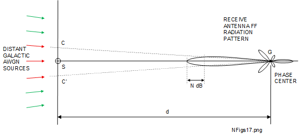
The example (far field) radiation pattern is of a satellite receive antenna at a ground location (\(G\)), operating at around 10 \(GHz\), its main lobe aligned with a satellite \(S\). Although it is shown in two dimensions, the beam is usually assumed to be close to axially symmetric in 3 dimensions. The shortest likely distance \(d\) between the ground station and a low earth orbit (LEO) satellite with the current technology would be a minimum of several hundred kilometers and in the far field. This may be verified using (5.3-1) to calculate the far field threshold distance. For example, the free-space wavelength \(\lambda\) at 10 \(GHz\) is 0.03 \(m\) and even a very large antenna of say 10 \(m\) diameter will have a far field distance of only about 7 \(km\).
The extent of the antenna capture area, assumed to be circular, is shown by the dotted lines \(GC\) and \(GC'\) in Figure 5.2-1. This depends on the shape (sharpness) of the main lobe of the antenna radiation pattern. Typically, the contour defining the beam edge will be specified as, say \(N \, dB\) below its maximum value which will correspond to a particular beamwidth. The red and green arrows represent AWGN sources within and outside the capture area respectively. These will comprise AWGN sources from distant stars. We know that AWGN is broadband so it will include power in the region of our example frequency of 10 \(GHz\) which will degrade the receiver \(SNR\). Only the red arrows represent AWGN sources which contribute to the antenna noise temperature. The green arrows represent sources not affecting this link as they will not be 'focussed' sufficiently by the antenna, being off-beam. Most of the AWGN sources are distant stars so their noise power flux density near the satellite is relatively small due to the effects of the inverse square law on the power flux density over such distances.
Modern parabolic reflector antennas for satellite communications links (not those used for restoration telemetry), typically 1 \(m\) to 2 \(m\) in diameter, will have gains in the order of 40 \(dB\) relative to an isotropic radiator (40 \(dBi\)) at a downlink frequency of around 10 \(GHz\) [27]. -3 \(dB\) beamwidths will be around \(1^\circ\), approximately circular beam pattern.
Figure 5.2-1 raises some interesting questions. The largest astronomical AWGN source to the Earth is of course the Sun which has a surface temperature of approximately 5700 \(K\). This represents a serious source of AWGN should the orbit position of the satellite, the ground station and the Sun, align. Fortunately, this is predictable with reasonable accuracy. For geostationary satellites, Sun noise episodes occur for 2 periods per year, typically a few minutes outage per day over 3 or 4 days. A few calculations using elementary trigonometery, the physics of black body radiation and the inverse square law will show that, when sun interference does occur, a \(1^{\circ}\) beamwidth antenna will capture most of the 'visible' area of the Sun which will 'swamp' the receiver with AWGN noise. If this did occurr, the noise temperature of the ground station receive antenna would approach 5700 \(K\) for that period. For orbiting (non-geostationary) satellites, such as those in low Earth orbits (LEOs), Sun interference can still occur when the alignment conditions are right. In general, the durations will be shorter but more frequent compared to geostationary satellites. Also there may be scope for mitigation, using Sun interference predictions to transfer services away from LEO satellites as they approach high-risk periods.
So what are the AWGN contributions from other stars? The nearest star to the Earth excluding the Sun is Proxima Centauri. Its diameter is about 15% that of the Sun, and its surface temperature is only about 2992 \(K\). But the most important difference is that its location is 4.25 light-years from the Earth, which I make at about \(4 \times 10^{16}\,m\) compared to \(1.5 \times 10^{11}\,m\) for the Sun to Earth distance. Some more elementary trigonometry will show that the angle subtended on the Earth by rays of electromagnetic radiation from Proxima Centauri is about \(3\times10^{-7}\) of one degree. Of course there will be many other star AWGN sources to account for at varying temperatures, diameters and distances, so sky temperatures are mapped continuously.
We will assume that the direction of the satellite is well clear of the Sun and the ground station and satellite antennas are accurately aligned. Small levels of AWGN will still be received from many stars that align with the antenna beam, all of them very distant. This, collectively, is known as cosmic background radiation and is used to provide evidence for the age of the Universe. In general, the powers of those AWGN sources which are captured are functions of the antenna elevation angle and will add to form an equivalent AWGN power which determines the antenna noise temperature [23]. Radio astronomy measurements including 10 \(GHz\) have covered the range 3 \(K\) to 100 \(K\). Therefore, an assumed worst-case antenna noise temperature of perhaps 120 \(K\) might be reasonable.
Satellites may be designed with either orthogonal linear polarization, circular polarization (RH and LH) or a combination of both. Good cross-polar isolation performance allows increased capacity through polarization diversity for signals operating in the same frequency band. The polarization of thermal noise (AWGN) received from stars has been researched in Radio Astronomy. There are many phenomina which contributions to polarization rotation in its long journey from the source stars through space. A reliable assumption is to assume that the polarization is random on arrival at the aperture of the receive antenna.
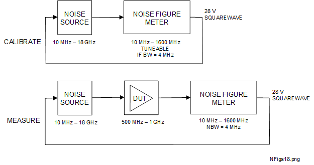
The Y-factor method is commonly used by NFMs and NFAs to provide a real-time readout of noise factor (and noise gain) after a suitable calibration procedure. For a DUT without frequency conversion operating within the frequency ranges of the noise source and the NFM, the calibration and measurement steps are shown schematically in Figure 5.4-1 [1] [17] [19].
The noise source is actually two AWGN sources, either of which may be switched to the output of the device, say at equivalent 'hot' and 'cold' noise temperatures of \(T_H\) and \(T_C\). Often, \(T_C\) is designed to be close to the local ambient temperature. To simplify calculations, it may be convenient to stabilise the ambient temperature to \(T_C = T_0 =290 \, K\) as this is frequently used in datasheets.
'Hot' and 'cold' refer to the greater and smaller equivalent noise temperatures of the noise source state respectively, selected by the 28 \(V\) on-off waveform which originates from the NFM. With a stable ambient temperature of 290 \(K\), then \(T_C=T_0 = 290 \,K\). This is a common test configuration which simplifies the ENR equation and will be used here. Applying this (3-7) for AWGN spectral noise power density (NPD), with \(T = T_0 =290\,K\), and converting to logarithmic units gives us -174 \(dBm/Hz\). To determine \(T_H\) for the same source, (5.4-1) is used with \(T_C=T_0 = 290 \,K\) and obtaining the value for \(ENR_{dB}\) from the noise source datasheet. For example, a common nominal \(ENR_{dB}\) is 14 \(dB\). Using this value and some manipulation of (5.4-1) gives us \(T_H = 7574 \, K\). Applying (3-7) again, but for this temperature, provides the NPD in this case of -160 \(dBm/Hz\), as expected, differing by \(ENR_{dB}\) from the \(T_0\) NPD.
The HP 346B noise source has quite a wide operating frequency range of 10 \(MHz\) to 18 \(GHz\). The precise ENR will typically vary by a few fractions of a dB across this range so an ENR against frequency calibration table is included with the device. Data from this may be programmed into the NFM before the measurement calibration to make the necessary minor adjustments. With the exception of the ENR table, all of the remaining discussion on Y-factor measurements will use linear units.
Y-factor is defined as the unit-less ratio of the power measured by the NFM in the \(T_H\) state (\(N_H\,\,watts\)) to the power it measures in the \(T_C\) state (\(N_C\,\, watts\)) (5.4-2). As the NFM itself controls the switching of the sources within the NS, it also stores each value separately in memory for later processing.
We know from the beginning of this section that we can replace a noisy device with a calculated equivalent input noise temperature and use a noise-free device with identical gain. This is the principle adopted for the Y-factor analysis. Therefore, with the (switched) noise source connected to the input of the DUT, the measured Y-factor of the DUT is given by (5.4-3) [1] [17] [19]:
Re-arranging (5.4-3) in terms of \(T_e\) gives (5.4-4).
Refer to the calibration schematic in Figure 5.4-1. For this example, the (Y-factor) noise factor measurement of a 2-port DUT without frequency conversion will be described. The ENR calibration data across the operating frequency range for the noise source to be used must be stored for processing in the NFM memory. The DUT has a frequency range of 500 \(MHz\) to 1 \(GHz\). This must be within range of both the noise source and the NFM RF input. The equations used for the equivalent noise temperature and noise factor for cascaded stages are shown in terms of noise temperature and noise factor in (5-8) and (5-9) respectively. Before the calibration, the NFM must be set to suitable start, stop and frequency steps and the other parameters set up according to the operating instructions [16].
Calibration must be performed with all of the necessary cables, connectors and adaptors, that will be required to connect the DUT output to the NFM input for the measurement, but excluding the DUT itself. The shortest possible cables and fewest adaptors connecting the noise source to the DUT after calibration must be allowed for. Ideally, the noise source connector type should be the same as the DUT input connector but of the opposite gender. If extra DUT input cables/connectors are unavoidable, their combined loss can be measured and then accounted for by entering the figures into the NFM under 'input loss compensation'.
After performing the calibration, the NFM will store the necessary data and indicate when calibration is complete. This procedure uses the Y-factor (\(Y_{2}\)) to measure the 'second stage' equivalent input noise temperature (\(T_{e2}\)) using (5.4-3), (5.4-4).
Furthermore, the NFM controls the switching of the noise source so it 'knows' when it is measuring \(N_H\) or \(N_C\) and can save them as required across frequency for later processing.
After calibration, whilst still stabilised, the DUT is connected as shown under 'measurement' in Figure 5.4-1. The same cables and adaptor arrangement that was used for the calibration must now be used for the DUT measurement.
The NFM will now measure the 'hot' and 'cold' noise powers for the cascaded stages 1 and 2 combined: the DUT (stage 1) and the remaining stages including cables, connectors and the devices within the NFM itself (stage 2). We will assume these powers are \(N_{C12}\) and \(N_{H12}\) respectively, then the gain of the DUT, the first stage only, \(G_1\) is given by (5.4-6):
Values for \(N_{C12}\) and \(N_{H12}\) also allow the instrument to calculate the Y-factor for the cascaded stages 1 and 2, \(Y_{12}\), similarly to (5.4-5), (5.4-6)
The final step is then to re-arrange the equation for the noise temperature of two cascaded stages (5-3) in terms of the noise temperature of stage 1, the DUT (5.4-7)
Thus the NFM is then able to calculate the equivalent input noise temperature of the DUT \(T_{e1}\) using the result for the gain of the DUT (\(G_1\)) from (5.4-6). Since we have used the standard noise temperature as a reference, the NFM may readily convert this to noise factor using (4.4-5).
Modern, high specification and very expensive, noise figure analyzers based on real-time digital signal processing (DSP), can perform measurements over many frequency ranges, bandwidths and modes of operation to high accuracy. However, our discussion is based on the Hewlett Packard (HP) 346B Noise Source and the HP 8970B Noise Figure Meter (NFM) [16]. This equipment was designed using the earlier superheterodyne architecture. The HP 8970B processing and download speeds are slower than those available with the DSP equipment but both generations still use the Y-Factor method that is described in Section 5.4.
The AWGN-based noise measurements to be described use the Y-factor method which is discussed in Section 5.4. Further to the discussion in Section 2 under 'Linear and Logarithmic Units', the parameters noise figure, noise factor and input noise temperature are synonymous. It is straightforward to convert between them. We will start with a simple noise figure measurement for a DUT without internal frequency conversion which is shown in Figure 5.5-1. The noise measurements must be performed under thermally stabilized conditions at an ambient temperature of 290 \(K\). The frequency range of the DUT, in this example 500 \(MHz\) to 1 \(GHz\), must be within range of both the noise source and the NFM RF input.
The NFM is designed to a low noise specification for measuring AWGN related parameters (noise figure, noise factor, equivalent input noise temperature and noise gain). It is possible for the HP 8970B to measure its own inherent noise figure using a suitable noise source, such as the HP 346B. I have measured this to be within the range 4 dB to 6 dB across 100 \(MHz\) to 1 \(GHz\). The instrument architecture is based upon a superhetrodyne design similar to a traditional (non-DSP) swept frequency spectrum analyzer. However the noise figures of spectrum analyzers are usually much greater than those of dedicated NFMs.
If the DUT operating frequency range extends beyond that of the NFM input, but still within the range of the noise source (for the HP346B this is 10 \(MHz\) to 18 \(GHz\)), then frequency conversion is required within the 'second stage' to bring it back to that range. This is frequency conversion, but external to the DUT. One example of the calibrate and measure configurations for a DUT frequency range of 4 \(GHz\) to 5 \(GHz\) with external frequency conversion is shown in Figure 5.5-2.
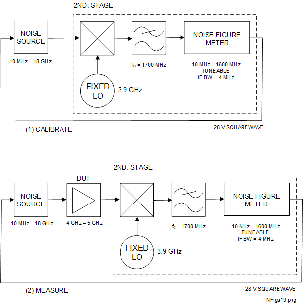
The mixer and fixed frequency local oscillator (LO) at 3.9 \(GHz\) will down-convert the DUT frequency band to the range 100 \(MHz\) to 1100 \(MHz\), suitable to connect to the NFM RF input. The mixer will generate another product of the noise source in the range 7.9 \(GHz\) to 8.9 \(GHz\) which is rejected from entering the NFM by the low pass filter (LPF) with a cutoff frequency of about 1700 \(MHz\). This may not be essential due to the input filtering of the NFM but is considered good practice. The 'second stage' now includes extra lossy parts (the LPF and mixer) before the NFM which will increase its noise figure compared to the non-internal frequency conversion case. There are some options for mitigating this which are described in the HP8970B user manual [16]. The NFM may be set up to include and compensate for suitable frequency offsets generated by the mixing process. In this case the LO is at a fixed frequency so the NFM frequency stepping capability is used to measure at frequencies across the DUT operating band.
An alternative to the fixed LO configuration shown in Figure 5.5-2 is the variable LO configuration which is shown in Figure 5.5-3
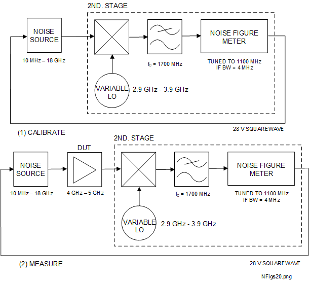
As an example, the LO may be tuned from 2.9 \(GHz\) to 3.9 \(GHz\) to give an IF output into the NFM at 1100 \(MHz\). The other mixing product would range from 6.9 \(GHz\) to 8.9 \(GHz\) so a similar LPF to that used for the fixed LO would be advisable. The LO frequency may be controlled either with an automatic test equipment (ATE) configuration or from the NFM itself if the facility is available. This method does have the advantage of allowing the NFM to be tuned to a lower IF such as 100 \(MHz\) where its noise performance may be better than closer to its upper frequency, 1600 \(MHz\).
Examples of DUTs with internal frequency conversion include mixers, receivers, upconverters and downconverters, in fact any 2-port device in which a swept input frequency does not produce an identical swept output frequency.
There are various options for measuring the noise figures of frequency converting DUTs. Knowledge of the DUT's intended operation, architecture and frequency planning is required to design an optimum (useful and reliable) test method. The examples shown are again featuring the HP 346B noise source and the HP 8970B NFM using the Y-factor method. For both instruments, extensive information is available online including theory, operating instructions, remote operation and examples [16].
Examples of calibration and some example measurement configurations for DUTs with internal frequency conversion are shown Figure 5.5-4 (1) to (4).
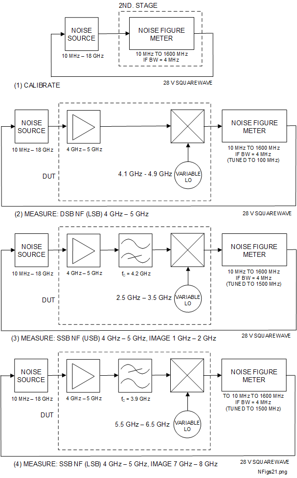
The HP 8970B has several set-up options for measurements on DUTs with internal frequency conversion. Once it 'knows' the intended measurement parameters (DSB, SSB, swept LO etc.) it calculates the frequency ranges needed for calibration and later measurement using the defined noise source and the loaded ENR table.
For double sideband (DSB) noise figure configurations, there are two AWGN paths through the mixer: the intended (signal) path and the image path. There is only one (wanted) path for the signal. The AWGN and wanted paths differ because signals are coherent, time-dependent and AWGN is random. The gain parameter \(G\) in the noise calculations is the small signal gain such as might typically be measured with a vector network analyzer (VNA), as opposed to the noise gain. By definition, the AWGN powers are additive, so the noise power arriving at the IF would typically be approximately twice that from either path separately. This assumes that there is no excessive slope of the ENR calibration between the two frequencies. It is also a function of any transmission (converstion loss) slope which may exist for the mixer. The best results are obtained if the IF (the frequency that the NFM is tuned to, 100 \(MHz\) in this case) is a small fraction of the LO frequency. Then there will likely be less variations of ENR or conversion loss between the wanted and image frequency paths. In this example, the LO frequency ranges from 4.1 \(GHz\) to 4.9 \(GHz\) so that both sidebands remain within the input frequency band 4 \(GHz\) to 5 \(GHz\). If measurements were required closer to the edges, the IF could be reduced to say 10 \(MHz\).
This example describes single sideband (SSB) via the upper sideband (USB) path. In this example, the DUT has been designed for an application with a high pass filter (HPF) before the mixer. The DUT uses a higher IF of 1500 \(MHz\) than the DSB case to provide more separation between the wanted and the image frequencies to make the high pass filter (HPF) design easier. The HPF is required to only allow one of the noise sidebands, in this case the USB, to be downconverted to the IF. Whilst the LO tunes from 2.5 \(GHz\) to 3.5 \(GHz\), the noise in the USB only is converted down to IF for measurement by the NFM. The HPF rejects any noise from the source which might get through the amplifier, despite it actually being designed for 4 \(GHz\) to 5 \(GHz\).
The same principles apply for this SSB (lower sideband, LSB) example as for the SSB (USB) measurement. Here, a low pass filter (LPF) rejects the USB from the noise source. Again, although this above the top operating frequency of the amplifier, it is good practice to include in case of any unwanted transmission through the device.
An example of a low noise cascaded receiving system devised by Pozar is shown schematically in Figure 6-1 [1] [2].
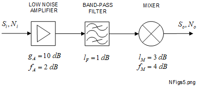
The local oscillator feeding the mixer is not shown. The first 3 stages of the receiver comprise a low noise amplifier (LNA), a bandpass filter and a mixer, each stage with the logarithmic gain (\(g\)), loss (\(l\)) and noise figure (\(f\)) shown in \(dB\). Each symbol has an appropriate subscript. An antenna with an input noise temperature of \(T_A = 150 \,K\), feeds the LNA input. The linear input signal and noise powers are \(S_i\) and \(N_i\) in watts. The linear output signal and noise powers are \(S_o\) and \(N_o\) in watts. The noise bandwidth of the cascade is determined by the passband response of the bandpass filter at 10 \(MHz\). All devices are well matched to the characteristic impedance which is 50 \(\Omega\) and are in thermal equilibrium at \(T_0 = 290 \, K\). The device noise figures were measured with an input temperature also at \(T_0\). The minimum SNR required at the output for the required quality of service is 20 \(dB\).
The second stage, bandpass filter, in Figure 6-1, has an in-band loss of 1 \(d B\). That is equivalent to a logarithmic in-band gain (say \(g_{F}\)) of -1 \(d B\). As the devices are in thermal equilibrium and well matched to the nominal system impedance of 50 \(\Omega\), the noise figure in \(d B\) will be the same as the in-band loss, just like an attenuator described in Section 4.6, so \(f_F\) = 1 \(dB\). These values will be converted to their linear equivalents using upper case symbols and the same subscripts for use in the equations. In summary, using Figure 6-1 and the equations (2-1), (2-2) and (2-3), we have the following linear values:
These are shown in Table 6-1.
| LNA (Stage 1) | BPF (Stage 2) | Mixer (Stage 3) | |||||||||
|---|---|---|---|---|---|---|---|---|---|---|---|
| \(g_A \, \, (d B) \) | \(G_A\) | \(f_A \, \, (d B) \) | \(F_A\) | \(g_F \, \, (d B) \) | \(G_F\) | \(f_F \, \, (d B) \) | \(F_F\) | \(g_M \, \, (d B) \) | \(G_M\) | \(f_M \, \, (d B) \) | \(F_M\) |
| 10 | 10 | 2 | 1.585 | -1 | 0.794 | 1 | 1.259 | -3 | 0.501 | 4 | 2.512 |
The defined bandwidth is 10 \(MHz\), applicable for the input and output noise powers, \(N_i\) and \(N_o\) respectively. There is a single frequency conversion, implied by the use of one mixer. The BPF could have been positioned at the output: assuming the same bandwidth but with a modified center frequency appropriate to the frequency conversion. This would make it clear that no AWGN is included outside of the passband of the BPF. In the present configuration, some AWGN from the mixer beyond the limits of the BPF would be present at the output. We will assume this is negligible.
The LNA would have been designed for a specific operating bandwidth appropriate to the signal band to be received. This is not specified so we assume that all the necessary filtering is done by the BPF at the input frequency. The antenna noise temperature of 150 \(K\) implies that it might be a satellite antenna. If it was, the frequency range could be in the order of several gigahertz so the percentage bandwidth would be very small.
The BPF could be positioned before or after the LNA. Each case has advantages and disadvantages. Placing it before the LNA reduces the risk of non-linear effects (intermodulation products and harmonics) but increases the overal noise figures as the front end logarithmic loss of the BPF adds to the system noise figure. Placing it after the LNA gives a better noise figure performance but opens the LNA to potentially more sources of intermodulation distortion.
To calculate the total linear gain of the cascade, the individual linear gains may be multiplied as shown in (6-1).
Alternatively, the individual logarithmic gains could be added (6-2) to give the overall logarithmic gain, say \(g_T\).
Using the parameter summary shown in Table 6-1, we will determine the equivalent gain and noise factor of the cascaded stages. The equivalent linear gain, say \(G_T\), is the product of the linear gains (6-1).
The noise factor of the 3 cascaded stages may be calculated from Friis's formula 6-3 which applies under thermally stable conditions at at a temperature of 290 \(K\), for closely matched 2-port devices.
The total noise factor \(F_T\) is expressed as a function of the noise factors of stages 1, 2 and 3 and the linear gains of stages 1 and 2. Provided the cascade is operating under the specified conditions, Friis's formula enables the cascade to be converted to an equivalent 2-port device with linear gain \(G_T\) and noise factor \(F_T\). One of those conditions is temperature defining the input AWGN level, in this case 290 \(K\).
If required, this may be converted to the logarithmic equivalent of noise figure using (2-4).
The schematics in Figure 6-2 show the steps necessary to arrive at this result.