The Hertzian Dipole and the Spherical Co-ordinate System

The best way to mathematically represent the electric and magnetic fields produced by a Hertzian Dipole (HD) is to use a spherical coordinate system which we will look at before we get to Maxwell's Equations. Although the HD is not a point source, it does have a finite length in one dimension, most commonly defined as coincident with the z axis. That length is used to relate the actual length of a real HD to the wavelength of the radiation which feeds it. As we have seen, the actual length must be much less than the wavelength of the radiation in use.

There are many conventions for spherical coordinates used in physics, navigation and mathematics which have evolved over the years, so where do we start? Later, we will be looking at how they apply to antenna describing radiation patterns in particular, so I will use what I believe is the most common usage in those specialisations. If you would like to study spherical coordinate systems in further depth, there is a well developed Wikipedia article on the subject.

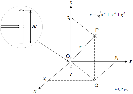
The dipole is assumed to be fed from a perfectly balanced, loss-free transmission line which does not influence its performance. Figure 1-1 shows a common definition of how the HD may be orientated within the rectangular (or Cartesian, \(x,y,z\)) coordinate system. The HD axis is aligned with the \(z\) axis with its mid-point co-incident with the \(xy\) plane. A time-varying sinusoidal current of instantaneous value \(I\) is fed through the HD in the direction shown. The radiated field from the HD is seen by an observer located at an arbitrary point \(P\). The position of \(P\) is described by the rectangular coordinates of the form \((x\,,y\,,z)\), such as \((x_1\,,y_1\,,z_1)\). Therefore, the straight line distance from the origin to \(P\) (\(OP\)) is given by (1-1).

\[r=\sqrt{x^2+y^2+z^2}\]

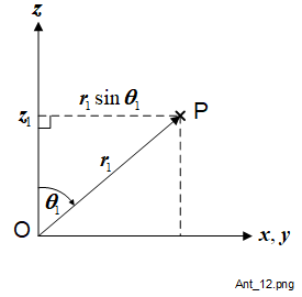
A common definition of the spherical coordinate system, which we shall be using, is shown in Figure 1-2 where the distance \(r\) and the angles \(\theta\) and \(\phi\) are defined. The center of the spherical coordinate system is coincident with the origin used for the rectangular coordinate system.

The HD is positioned at the origin. The fields generated by the HD will be complicated functions of distance and direction derived from Maxwell's Equations. The spherical coordinate system has been developed to allow various simplifications to be applied using Maxwell's Equations on account of the axial symmetry of the HD.

It is very useful to be able to convert between the two coordinate systems for describing the electric and magnetic vector fields generated by the HD exactly in magnitude and phase at any arbitrary point P.

To describe these vectors we will include an arrow above the vector symbol pointing to the right, for example \(\overrightarrow{E}\) and \(\overrightarrow{H}\) for the electric and magnetic (vector) fields respectively. Alternatively, sometimes conventions use bold type for vector symbols and normal type for scalar symbols. Arrows and similar symbol add-ons are useful for manuscript and may be more readily identified from blocks of text. We will use the general vector symbol \(\overrightarrow{A}\), as applicable to either of these vectors. Refer now to Figure 1-2 which shows the associations of the rectangular and spherical vector definitions that we will be using.

In Figure 1-1 we saw how the position of point P could be represented in rectangular coordinates by \((x_1\,,y_1\,,z_1)\). Figure 1-2 shows how it may also be represented in spherical (\(r,\,\theta,\,\phi\)) coordinates. Both spherical and rectangular coordinates can be used to specify a position anywhere in 3 dimensions, but the position information is scalar only. To start with, we are only considering position, the position of the observer, information for which elementary three dimensional trigonometry will suffice. Vectors will come shortly but we have to first specify the position of the vector.

We will recall that the surface of the Earth itself is approximately spherical. The latitude and longitude navigational coordinate system is almost identical to the spherical coordinate system we have chosen. If our \(z\) axis is coincident with the Earth's polar axis and the \(x,\,y\) plane is in the Earth's equatorial plane, the origin is at the center of the Earth, \(\theta\) is similar to latitude and \(\phi\) is similar to longitude. Of course we use different angle references for navigation on or near the Earth's surface.

The straight line distance (\(r\)) from the origin O to P, say OQ, is given by (1-1). The angle in the \(x\,,y\) plane between the \(x\) axis and the projection of OP to OQ is defined as \(\phi\). The angle between the \(z\) axis and OP is defined as \(\theta\).

Although it may not be immediately obvious from Figure 1-2, we use a different definition to those used for the Earth's latitude and longitude. The ranges of \(\theta\) and \(\phi\) are chosen to cover the whole space without any overlapping, given by (1-2).

\[0\le\,\theta\,\le\,\pi\] \[0\le\,\phi\,\lt\,2\pi\]

Do We Really Need Infinite Points and Negative Radii?

When writing code for using trigonometrical equations such as these, some caution may be required in dealing with the compound angles for \(\theta\) and \(\phi\). For example, (1-4) and (1-5) are the inverse cosine and inverse tangent formulas for \(\theta\) and \(\phi\) respectively. Taking the former, the built-in Matlab 2023a® function arc-cosine (acos()) gives the result 150° for acos(-0.866). Of course, within the first 4 quadrants, the other result is 210°. Fortunately that is not relevant here because \(\theta\) does not extend beyond 180°.There are of course an infinite number of quadrants and therefore an infinite number of such angles and that is just in 2 dimensions. If you really want to research spherical coordinate systems in more depth, I suggest you start with that Wikipedia article which I referenced earlier. In the following discussion we will consider formulas for the cases when the rectangular coordinates are all positive.

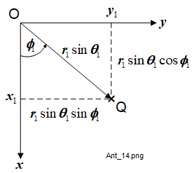
Some elementary 3-dimensional trigonometry based on the coordinate systems shown in Figure 1-1 and Figure 1-2 with the help of Figure 1-3 and Figure 1-4 will relate the position of P to either the rectangular coordinate system \((x_1\,,y_1\,,z_1)\) or the spherical coordinate system, say \((r_1\,,\theta_1\,,\phi_1)\).

We now have 3 equations which describe the position information which may be used to convert between the 2 coordinate systems: (1-1) repeated below, (1-4) and (1-5).

\[r=\sqrt{x^2+y^2+z^2}\]

\[\theta=\cos^{-1}{\left(\dfrac{z}{r}\right)}\]

\[\phi=\tan^{-1}{\left(\dfrac{y}{x}\right)}\]

(1-1), (1-4) and (1-5) may be used to readily convert the position in rectangular coordinates to spherical coordinates.

To convert the position from spherical to rectangular coordinates, re-arranging (1-4) gives the equation for \(z\) (1-6). Then solving (1-1) and (1-5) for \(x\) and \(y\) results in

\[z=r\,cos\theta\]

\[x=r\,sin\theta\,cos\phi\]

\[ y=r\,sin\theta\,sin\phi\ \]

Vector Representations

So far with the rectangular and spherical coordinate systems, we have just considered the position of the measurement point P. A practical vector field will probably be non-uniform with typically the source located at the origin. That is probably why we want to measure it, so the positions of the 'observers' must be defined unambigously. We can define the position of P in either coordinate system as we know the relationship between them and can convert as necessary. We will now consider the vectors themselves, expressed using both coordinate systems. For practical antennas, the fields they generate are usually functions of the straight line distance and orientation of the observer from the source. In this case the source is not a point, as might be the assumption with an isotropic radiator but, as we have seen, a Hertzian Dipole: a small cylindrical element which has axial symmetry and is coincident with the \(z\) axis.

Referring again to Figure 1-2, note the short component vectors for the two systems, shown in red. These are unit vectors. The unit vectors for the \(x,\,y,\,z\) axes are \(\hat{x},\,\hat{y},\,\hat{z}\) respectively; and for the \(r,\,\theta,\,\phi\) axes they are \(\hat{r},\,\hat{\theta},\,\hat{\phi}\) respectively. The components are equivalent to the vectors in each of the 3 dimensions. For both coordinate systems, each dimension is orthogonal to the other two vectors and such a vector is the sum of its component vectors. They will have identical units because we already know each of their directions.

Electromagnetic fields can either be electric \(\overrightarrow{E}\) or magnetic \(\overrightarrow{H}\). Maxwell's Equations tells us that propagating fields such as these must be time-varying and sinusoidal. The SI unit representation for the electric and magnetic fields would be volts per metre (V/m) and amperes per metre (A/m) respectively. They will be sinusoidally varying with time so we have to specify which sinusoidal parameter is being used, for example root mean square (RMS) or peak.

Any 3 dimensional vector is equivalent to the sum of three separate component vectors, each component representing one dimension. We will represent a vector using rectangular and spherical components as (\(\overrightarrow{A_{xyz}}\)) and (\(\overrightarrow{A_{r\theta\phi}}\)). The general forms of these are shown in (1-3) and (1-4) respectively. To re-iterate, in each case the 3 component vectors are always mutually at right angles.

\[\overrightarrow{A_{xyz}}= A_x\,\hat{x}+A_y\,\hat{y}+A_z\,\hat{z}\]

\[\overrightarrow{A_{r\theta\phi}}= A_r\,\hat{r}+A_{\theta}\,\hat{\theta}+A_{\phi}\,\hat{\phi}\]

Note that in (1-4) the radial magnitude \(A_r\) is, by definition, along the radial line OP. It is not a radius scalar so it can be negative. For each vector component, the vector itself is the product of the magnitude and the associated unit vector. The magnitude is a scalar quantity but product of it and the assoicated unit vector changes it to a vector. These apply precisely in the directions of their associated component axes as shown by the arrows.

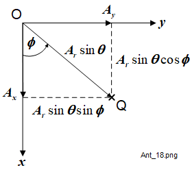
The symbol for each scalar is often the same or similar to that for the the resultant vector but with subscripts according to the coordinate system, for example, \(x\), \(y\) and \(z\) for rectangular coordinates. These are shown adjacent to the extensions of the unit vectors in Figure 1-4. For example \(A_x\) for \(\hat{x}\) and \(A_\phi\) for \(\hat{\phi}\).

Vector Conversions

To convert a vector between rectangular and spherical coordinates, refer again to Figure 1-2. This shows the rectangular components acting at the origin (O) and the spherical components at point P. Whilst we must always unambigously define the position of the 'observer', in this case the points O and P are different simply to avoid cluttering the diagram. Either vector could be anywhere in the 3 dimensional space but always at a defined position. We know that the vector component magnitudes are \(A_x\), \(A_x\), \(A_y\) for the rectangular vector and \(A_r\), \(A_\theta\), \(A_\phi\) for the spherical vector.

Consider first conversion of a rectangular vector \(\overrightarrow{A_{xyz}}\) to a spherical vector \(\overrightarrow{A_{r\theta\phi}}\). The vector equations for these are (1-3) and (1-4) respectively.

We need to calculate the contribution of the rectangular components to the spherical components by applying elementary 3 dimensional trigonometry algebraically and very carefully using the definition shown in Figure 1-2. In the following figures I have extracted some of the 2 dimensional planes to help. To simplify the calculations, we will assume that the vectors are located at the origin, but of course they can be anywhere.

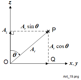
In Figure 1-5 and Figure 1-6 the \(A_r\) scalar component (OP) is considered with its projection on to OQ in the \(x,\,y\) plane, also its component in the \(z\) axis direction.

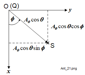
In Figure 1-7 and Figure 1-8 the \(A_\theta\) component, say PR, is considered with its projection, say QS, to the \(x,\,y\) plane and its \(z\) component in the same plane as the \(z\) axis.

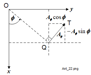
And finally, Figure 1-9 shows the \(A_\phi\) scalar component projection (say QT) viewed in the \(x,\,y\) plane and resolved into its \(A_x\) and \(A_y\) components. As \(A_\phi\) is defined as being only in the \(x,\,y\) plane, the \(A_z\) component is zero.

We can now simply add the \(x\), \(y\) and \(z\) component contributions for \(A_r\), \(A_\theta\) and \(A_\phi\) algebraically, allowing for the vector directions as well as magnitudes. The results are combined into a matrix equation in (1-5).

\[\begin{pmatrix} A_r \\[0.3em] A_\theta \\[0.3em] A_\phi \\[0.3em] \end{pmatrix}= \begin{pmatrix} sin\theta\,cos\phi & sin\theta\,sin\phi & cos\theta \\[0.3em] cos\theta\,cos\phi & cos\theta\,sin\phi & -sin\theta \\[0.3em] -sin\phi & cos\phi\ & 0 \\[0.3em] \end{pmatrix} \begin{pmatrix} A_x \\[0.3em] A_y \\[0.3em] A_z \\[0.3em] \end{pmatrix}\]

(1-5) shows that \(A_r\), \(A_\theta\) and \(A_\phi\) are functions of \(A_x\), \(A_y\) and \(A_z\), but also of \(\theta\) and \(\phi\) for the spherical definition.

To convert from spherical coordinates to rectangular coordinates, we may use a similar method, and the result is (1-6).

\[\begin{pmatrix} A_x \\[0.3em] A_y \\[0.3em] A_z \\[0.3em] \end{pmatrix}= \begin{pmatrix} sin\theta\,cos\phi & cos\theta\,cos\phi & -sin\phi \\[0.3em] sin\theta\,sin\phi & cos\theta\,sin\phi & cos\phi \\[0.3em] cos\theta & -sin\theta\ & 0 \\[0.3em] \end{pmatrix} \begin{pmatrix} A_r \\[0.3em] A_\theta \\[0.3em] A_\phi \\[0.3em] \end{pmatrix}\]

You may wish to work through these and hopefully confirm that (1-6) is correct.

Some Examples

Table 1-1 lists some conversions between the rectangular and spherical coordinate systems for defining positions relative to the origin. These are not vectors but simple scalar positions. The units are arbitrarily chosen. They are not important provided they are used consistently. Similarly the angle units are radians (rad) with degrees (deg) included for convenience.

Table 1-1 Rectangular to Spherical Coordinate Position Conversions

Rectangular			Spherical
x (m)	y (m)	z (m)	r (m)	\(\theta\) (rad)	\(\phi\) (rad)	\(\theta\) (deg)	\(\phi\) (deg)
1.00	2.00	3.00	3.74	0.64	1.11	36.7	63.4
4.00	-7.00	2.00	8.31	1.33	5.23	76.1	299.7
-1.00	-8.00	-5.00	9.49	2.13	4.59	121.8	262.9
-3.00	12.0	7.00	14.2	1.06	1.82	60.5	104.0
12.0	3.00	-15.0	19.4	2.45	0.25	140.5	14.0

Table 1-2 lists the same rectangular coordinates used for Table 1-1, but also some arbitrarily chosen rectangular vector component magnitudes \(A_x\), \(A_y\) and \(A_z\) and the equivalent spherical components, \(A_r\), \(A_\theta\) and \(A_\phi\).

Table 1-2 Some arbitrarily chosen vectors expressed in rectangular and spherical coordinates at various positions defined by rectangular coordinates. The positions may be related to the equivalent spherical coordinates from Table 1-1.

Rectangular Position (m)			Rectangular Vector (V/m)			Spherical Vector (V/m)
x (m)	y (m)	z (m)	\(A_x\) (V/m)	\(A_y\) (V/m)	\(A_z\) (V/m)	\(A_r\) (V/m)	\(A_\theta\) (V/m)	\(A_\theta\) (V/m)
1.00	2.00	3.00	3.00	4.00	5.00	6.95	0.96	-0.89
4.00	-7.00	2.00	-10	6	-32	-17.6	28.6	-5.7
-1.00	-8.00	-5.00	97	21	-32	-11.1	44.5	93.6
-3.00	12.00	7.00	22	9	367	183.7	-317.7	-23.5
12.00	3.00	-15.00	5	23	-4	9.7	-5.5	21.1

• Return to Top
• Return to Chris Angove's Home Page