Electrical Connections Without Wires: Wireless

In the mid-seventeenth century, Pieter van Musschenbroek of Leyden (1692-1761) built a device which was later named 'The Leyden Jar', a predecessor of the modern capacitor and a component capable of storing electrical charge. The Leyden Jar comprised two uniformly spaced conducting plates separated by an insulator which formed the glass part of the jar. Electrical connections to the plates were made with metal wires.

The Galvanometer, an instrument designed for measuring small electric currents, was named after Luigi Galvani (1737 - 1798). Galvani demonstrated that small electrical currents could be carried by wires constructed from metal like those used to connect to the plates of the Leyden Jar. To this day we use the adjective 'Galvanic' to describe the connection using an electrical conductor through which an electrical current can flow.

The experiments on electromagnetic induction conducted by Michael Faraday (1791 - 1867) showed that electrical pulses, measured with a galvanometer, were detected when a magnetic field 'linked' with a coil of wire was quickly changed. Schematics of Faraday's experiments are shown in Figure 1-1.

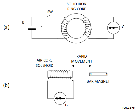
In neither of Faraday's experiments was there a Galvanic connection between the 'source', the battery for (a) or the magnet for (b), and the galvanometer. In modern technology we might refer to the galvanometer as the 'load'. In (a), although the ring core was constructed from iron which was known to be an electrical conductor, wires forming the coils were insulated from each other and from the core by woven cotton. In those days iron was often used as an electrical conductor, with or without insulation, because it was readily available and cheap. Today we would consider it a poor choice because of its relatively high resistivity creating resistance and wasting significant power. Although copper had been discovered from about 8000 BC, it was scarce and expensive and it would be many years before large scale mining of the ores and the extraction of the metal itself would bring the prices down. Although aluminium had recently been discovered, it is only in recent years that it has become economic to extract the metal from the ore in large volumes.

The Non-Galvanic Connection

In those early days of electrical engineering, it was clear to many scientists that the Galvanic connection was not always necessary to demonstrate some sort of 'stimulus' and 'response' across one or more insulators, glass for the Leyden Jar and cotton for Faraday's experiments. It was known that the atmosphere was also a good insulator but unfortunately the dimensions involved were orders of magnitude greater than those applicable to the glass or the cotton, so there were some challenges ahead before it could be used for long distance communications.

Early scientists were familiar with the properties of magnetism after reading the works by William Gilbert, a physician (1544-1603) who wrote several books on the subject called De Magnete. Around the same time William Sturgeon (1783-1850) invented the first electromagnet, which was a device designed to create magnetism from electricity. So it was known that, under the right conditions, electricity could create magnetism and magnetism could create electricity, again with no Galvanic connection between the source and the load. The problem was that this only occurred if there was physical movement between a source and a load (or destination). After further work it was demonstrated that, if the source and load were in fixed positions, the electrical currents (or charge flows) of the source over time induced some similar changes of the currents in the load, again over time, which appeared arbitrary. These observations demonstrate properties of the early transformer.

Otto Blathy (1860-1939) invented the modern, high efficiency transformer. If all of its modern evolutions are included, probably millions of transformers of many different types are used today all over the World. Their applications are not just for relatively high power transmission but also for many electronic situations across vast frequency ranges including: communications equipment, radar, modern high efficiency power supplies and digital cellular terminals.

So what possible use would there be for electricity as some form of communication and how may it be transferred from one place to another? Could it even be transmitted in some way without wires? The two schematics in Figure 1-1 show the situation that the scientists of the early nineteenth century were facing. The voltage from a source with some, as yet little understood, variation with time may be transferred to a load at the destination on the right. The top circuit achieves this using the electric fields within capacitors and the bottom circuit using the magnetic fields within a transformer. The connections between the devices at either end were Galvanic but the media between each end in each case were insulators.

So there were apparently two alternative methods of transferring electrical impulses from a source to a load, but neither of which required a direct Galvanic connection between the source and the load. That was because the capacitors included insulators as dielectrics and the transformer comprised two windings which were Galvanically isolated from each other by air or another insulator such as cotton. Unfortunately, in both cases the thickness of the non-Galvanic portion which we might say is 'in the direction of propagation', was only a few millimetres at most so would not have been much use communicating wirelessly across countries. However, realising the great potential for 'wireless' (non-Galvanically connected) communications, in some way using electric and/or magnetic fields after some further development, the scientists proposed the presence of an 'Aether', or a medium, not yet fully understood, to carry the necessary electric voltages or currents through insulators, which might include the atmosphere.

Maxwells' Equations and Hertz's Verifications

Eventually, the necessary mathematical proof that time varying waves with both electric and magnetic properties, electromagnetic or EM waves, can propagate 'through the air' and even through the near vacuum of space, was provided by the physicist and mathematician, James Clerk Maxwell (1831-1879). Maxwell's work showed that EM waves were possible and would propagate through free space, a perfect vacuum, at the speed of light, just like visible light which was also a form of EM radiation. The time varying requirement of EM waves means they had to be alternating sinusoidally, so they required some form of oscillatory circuit to generate them.

Maxwells' Equations, using modern mathematical operators and calculus symbols are shown in point (differential) form and integral form in Table 1-1. The right column suggests alternative names for each to avoid possible ambiguity of simply numbering them. Oliver Heaviside was responsible for simplifying them from the original (20 equations and 20 unknowns) into this form, the most widely used today.

Table 1-1 Maxwell's Equations in differential form, integral form and alternative names

Maxwell (Differential Form)	Maxwell (Integral Form)	Alternative Name
\[\nabla \bullet \boldsymbol{E}=\frac{\rho}{\epsilon_0}\]	\[ {\Huge \unicode{x222F}_{\normalsize S }} \boldsymbol{E} \bullet d \boldsymbol{S} = \frac{1}{\epsilon_0} \iiint_V \rho \, d V \]	Maxwell-Gauss (Electric)
\[\nabla \bullet \boldsymbol{B}=0\]	\[ {\Huge \unicode{x222F}_{\normalsize S}} \boldsymbol{B} \bullet d \boldsymbol{S} = 0 \]	Maxwell-Gauss (Magnetic)
\[\nabla \times \boldsymbol{E}=-\frac{\partial \boldsymbol{B}}{\partial t}\]	\[ \oint_C \boldsymbol{E} \bullet d \boldsymbol{l} = -\frac{\partial}{\partial t} \iint_S \boldsymbol{B} \bullet d \boldsymbol{S} \]	Maxwell-Faraday (Induction)
\[\nabla \times \boldsymbol{H}=\boldsymbol{J} + \frac{\partial \boldsymbol{D}}{\partial t}\]	\[ \oint_C \boldsymbol{B} \bullet d \boldsymbol{l} = \mu_0 \iint_S \boldsymbol{J} \bullet d \boldsymbol{S} + \mu_0 \epsilon_0 \frac{\partial}{\partial t} \iint_S \boldsymbol{E} \bullet d \boldsymbol{S} \\ \]	Maxwell-Ampere (with Displacement Current Density)

All parameters indicated by an arrow are vector quantities. The others are scalar. The vector operators ∇• and ∇× represent divergence (div) and curl respectively. The symbols represent the following quantities:

• D: surface charge density in coulombs per metre squared (Cm^-2);
• ρ: volumetric charge density (scalar) in coulombs per metre cubed (Cm^-3);
• B: magnetic flux density in tesla (T) or webers per square metre (Wbm^-2);
• E: electric field strength in volts per metre (Vm^-1);
• t: time (scalar) in seconds (s);
• H: magnetic field strength in ampere per metre (Am^-1);
• J: current density in ampere per metre squared (Am^-2).

Much of Maxwell's work was to rationalise and co-ordinate the work of earlier scientists, especially Gauss, Faraday and Ampere. A brief explanation of each of his differential equations follows:

• $\nabla •\overrightarrow{D}=\rho$

  This is the differential form of Gauss's Law which is equivalent to $\nabla •\overrightarrow{E}=\rho /\epsilon$, where ε is the permittivity of the medium. This states that the divergence of the electric field is proportional to the charge density.

• $\nabla •\overrightarrow{B}=0$

  Also known as Gauss's Law for Magnetism, this states that the divergence of a magnetic field is zero as it is solenoidal (it exists in loops). That is equivalent to the statement that magnetic monopoles do not exist (for every north pole there is a south pole and vice versa).

• $\nabla \times \overrightarrow{E}=-\frac{d\overrightarrow{B}}{dt}$

  This is the equivalent of Faraday's Law of Electromagnetic Induction. Included in Faraday's many experiments were versions which demonstrated that a change in the flux linking a magnetic field and a circuit comprising a loop of conductive wire connected to a galvanometer caused an electric current. The change was a function of time and could be achieved by moving the relative positions of the loop and the magnetic field. Alternatively, their relative positions could be fixed and the current could be momentarily changed for example by switching it on and off. The negative sign on the right hand side of the equation resulted from Lenz's Law. Lenz found that the direction of the induced voltage was in the direction such as to oppose the field changes causing it.

$\nabla \times \overrightarrow{H}=\overrightarrow{J}+\frac{\partial \overrightarrow{D}}{\partial t}$

Ampere's classic Circuital Law was originally derived by Maxwell using hydrodynamics in 1861. In 1865 he modified Ampere's equation to include a displacement current, the$\partial \overrightarrow{D}/\partial t$ term. The displacement current density has the same units as electric current density and both are sources of magnetic fields. In physical materials as opposed to free space, there is also a contribution from dielectric polarization.

Many of the leading academic and industry references on electromagnetic theory have comprehensive sections on Maxwell's equations and just about everything associated with them. For a full mathematical workout of these from sources other than Wikipedia, consult for example: Kraus and Carver, Pozar, Stutzman & Thiele or Ramo, Whinnery and Van Duzer.

The physicist, Heinrich Rudolf Hertz (1857-1894) was the first scientist to conclusively prove the existence of electromagnetic waves that were predicted by Maxwell. In recognition of Hertz's work, the SI unit of frequency, one cycle per second, was renamed the hertz (Hz) in 1960. Units named after scientists is rather like statues: they are usually very worthy and a great honour for those concerned, but posthumous.

As part of his Ph.D thesis at the University of Berlin, Hertz demonstrated some of the properties of directional antennas and propagation over a few metres: polarisation, reflection, refraction and standing waves, all of which had been predicted by Maxwell. Although, initially it was not named as such, Hertz is generally considered to be the inventor of the what we now call the wireless antenna [22]. Readers will also be interested to know that Hertz studied under Kirchhoff (1824-1887) and Helmholtz (1821-1894), famous for their circuit current laws and the Helmholtz Equation [23].

The actual frequencies used by Hertz have been estimated to be about 50 MHz and 450 MHz. The unit hertz may be used to describe the frequency of any periodic phenominia with respect to time. Perhaps the electrical sinusoidal variation of voltage or current with respect to time as used with EM waves is the most common. The basic configuration of Hertz's apparatus is shown in Figure 1-2.

What is an Antenna?

The schematic shown Figure 2-1 shows the key elements in a wireless link as it might have been demonstrated in teh early twentieth century.from a time varying source on the left to a load at teh destination on the right.