Why is Additive White Gaussian Noise so Important in Communications and Radar Systems?

Additive white Gaussian noise (AWGN) is generated within the imperfect components used in all electronic electronic circuits [2] [4] [5] [8]. It is present at all temperatures above absolute zero. The mean power level of AWGN is directly proportional to the product of two variables: the absolute temperature of the source and the noise bandwidth of the communications channel(s) which it affects. Therefore, the only measures available to minimise AWGN are: reducing the bandwidth and/or reducing the operating temperature. Its greatest influence is on communications and radar receiving equipment, especially the 'front end' stages where the received signal from an antenna or cable meets its first stage(s) of amplification. It is still present in other electronics hardware, but its relatively small amplitude usually makes it's effect insignificant compared to the signal levels present in normal operation.

The laws of physics tell us that the frequency range of AWGN covers to well in excess of the frequency range of radio equipment that exists with the current technology, to over 100 \(G H z\) [1] [3] [9]. AWGN voltage and phase components are random across frequency, so it cannot be filtered out and it is therefore always present with the signal. The best signal to noise ratio (SNR) performance with AWGN is achieved by minimising the AWGN power and maximising the signal power. The influence of AWGN is therefore greatest in the small signal stages at the front end of a receiver, typically fed by an antenna.

The Derivation AWGN from Black Body Radiation

For a resistor \(R\) ohms (\(\Omega\)) at an absolute temperature \(T \) kelvin (\(K\)), the random and independent motion of large numbers of electrons results in small random voltage fluctuations across the resistor. The AWGN average voltage is zero, but the mean square voltage is finite and proportional to the mean linear power for a given bandwidth. The root mean square (RMS) value of the noise voltage, \(V_n\) volts (\(V\)), is given by Planck's black body radiation law, (2-1) [1] [5].

\[V_n = \sqrt{\frac{4 h f B R}{e^{\frac{h f}{k T}}- 1}} \]

where:

• \(h\): Planck's constant, \(6.626 \times 10^{-34}\) joule seconds, \(J s\).
• \(k\): Boltzmann's constant, \(1.380 \times 10^{-23}\) joule/kelvin, \(J/K\).
• \(B\): the noise bandwidth of the source in hertz, \(Hz\).
• \(f\): the absolute frequency in hertz, \(Hz\).

Using a math application such as Matlab® or Excel® for example, (2-1) is plotted in Figure 2-1 for some arbitrary values of resistance \(50 \, \Omega\), temperature \(290 \, K\) and noise bandwidth \(1 \, GHz\) and across a frequency range \( 10 \, M H z \) to to \(100\, THz \). The vertical scaling is logarithmic in dB-microvolts (\(d B \mu V\)), defined as \(20 \log_{10} (v_n)\), where \(v_n\) is \(V_n\) expressed in microvolts, so \(v_n = V_n \times 10^6\).

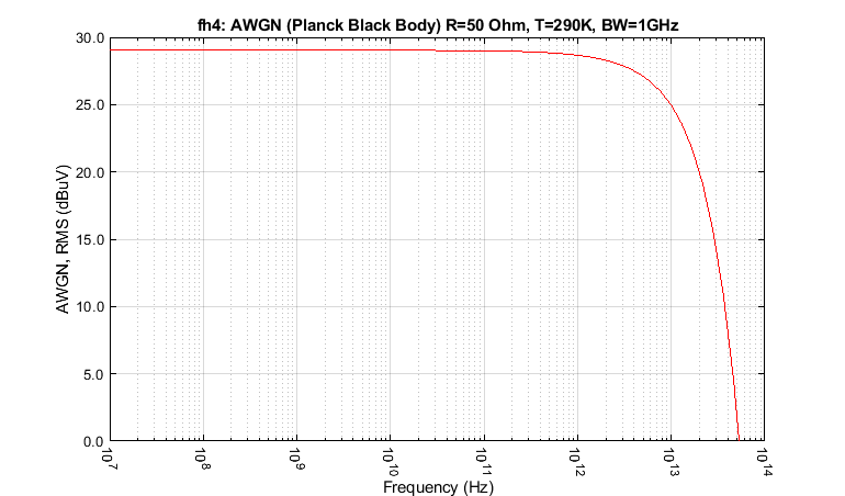
This shows the AWGN RMS noise voltage to be constant at about 29 \(d B \mu V\) to well beyond 100 \(G H z\). In fact, it does not start to fall significantly to well past 1000 \(G H z\). This shows the 'white' property of AWGN, the analogy being with the optical part of the electromagnetic spectrum.

In the RF and microwave frequency range, if we take the upper frequency as \(f = 100 \, G H z \) and the component at approximately room temperature \(T = 290 \, K\), then \(h f \, \ll k T \) is valid and the first 2 terms of a Taylor series gives (2-2):

\[e^{\frac{hf}{kT}}-1 \approx \frac{hf}{kT} \]

Using (2-1) and (2-2), results in (2-3)[1]. This method is also known as the Raleigh-Jeans approximation.

\[V_n = \sqrt{4 k T B R}\]

This equation is sufficiently accurate to use for all communications equipment using the current technology. For very low temperatures and/or very high frequencies, using (2-1) directly may be slightly more accurate.

We can show that the mean noise power \(P_n\) is not a function of resistance by creating a Thevenin equivalent circuit for the AWGN source with a noise-free source resistance \(R\) connected to a normal (noisy) load of resistance \(R\) via a perfect bandpass filter (BPF). This will transfer the maximum possible power from the source to the load and is shown in Figure 2-2. Practical electronic parts would always be band limited so the BPF is necessary to define the applicable equivalent bandwidth of AWGN, \(B\) in (2-3), otherwise the noise power would theoretically be infinite [2] [4]. The BPF in has a hypothetical 'brick wall' frequency response: 100% transmission (zero insertion loss) in the transmission band \(f_1\) to \(f_2\) and zero transmission outside of this band.

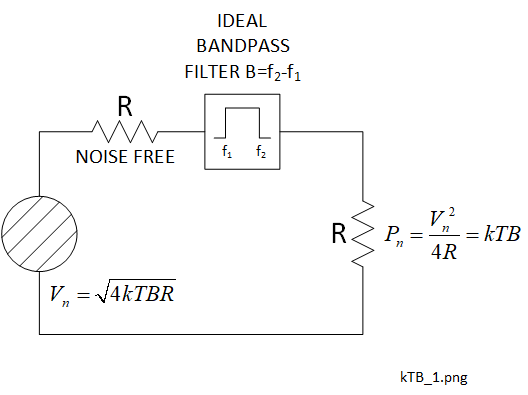
The mean AWGN noise power in the load resistor, \(P_n \) watts (\(W\)) is therefore given by (2-4).

\[ P_n = k \, T B \]

Gaussian Distribution of the Random Noise Voltages

AWGN is the result of large numbers of independent electron charges in random motion. The Gaussian property originates from the Central Limit Theorem [4] [5]. The voltage generated from each charge may be represented as a voltage vector whose amplitude and phase are also random. The resulting noise voltages will interact with each other according to their time and phase relationships. The instantaneous phase values will be uniformly distributed between 0 and 2\(\pi\) radians. The resultant noise voltages will have a Gaussian distribution with a mean value of zero.

(3-1) represents the probability density function (PDF) for a Gaussian distribution of an independent random variable \(x\) with a mean \(\mu\) and standard deviation \(\sigma\). For AWGN, \(x\) relates to the values of the noise voltages for a band-limited range of frequencies [2] [6] [10].

\[p(x) = \frac{1}{\sigma \sqrt{2 \pi}} exp{\left( - \frac{1}{2} \left( \frac{x - \mu}{\sigma} \right)^2 \right)} \]

A special case of the PDF is the normalised form of (3-1) with a mean of zero (\(\mu = 0 \)) and a standard deviation of one (\( \sigma = 1 \)). This is shown in (3-2).

\[ p(x) = \frac{1}{\sqrt{2 \pi}} exp{\left( - \frac{x^2}{2} \right) } \]

(3-2) is plotted in Figure 3-1. To consider the AWGN power, we start with the normalized Gaussian distribution function. In this case the mean is zero (\(\mu = 0 \)) and the standard deviation is 1 (\(\sigma = 1\)) for the normalized condition, so (3-1) becomes (3-2).

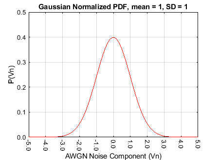
As the variance is the square of the standard deviation, these values will both be numerically equal to one (\(\sigma^2 = \sigma = 1 \)) for the normalised case. For an absolute (un-normalised) example, we will also need to account for the units necessary for the variance and the standard deviation. The normalized condition means that the area under the curve is equal to one because the voltage range is nominally from \(- \infty \) to + \( \infty \), so every voltage must be included. If we apply this to AWGN, '\(x\)' becomes the spread of independent noise voltages from the electrons charges and also has a mean of zero. Furthermore, the band limited normalized AWGN (mean) noise power is equal to the variance of the distribution.

To relate the Gaussian PDF to an un-normalized version of AWGN, we may examine the following band-limited example: a noise bandwidth (\(B_N\)) of 100 \(M H z\), an absolute temperature (\(T\)) of 290 \(K\) and a load resistance (\(R\)) of 50 \(\Omega\). The mean AWGN power \(P_n\), using (2-4) is \(4 \times 10^{-13}\) \(W\). The mean square AWGN voltage, \(V_{M S}\) (3-3) and the RMS AWGN voltage, \(V_{R M S}\) (3-4) are equivalent to the variance (\(\sigma^2\)) and the standard deviation (\(\sigma\)) respectively.

\[V_{M S} = P_n R \]

\[V_{R M S} = \sqrt{P_n R} \]

So, for our example, using (3-3) for the variance and (3-4) for the standard deviation, we have \(\sigma^2 = 2 \times 10^{-11}\,\, V^2\) and \(\sigma = 4.4 \times 10^{-6}\,\,V \). We can then de-normalise the Gaussian independent variable \(x\) axis using \(\sigma = 4.4 \times 10^{-6}\,\,V\). This will also de-normalize the area under the PDF. The result of this is shown in Figure 3-2.

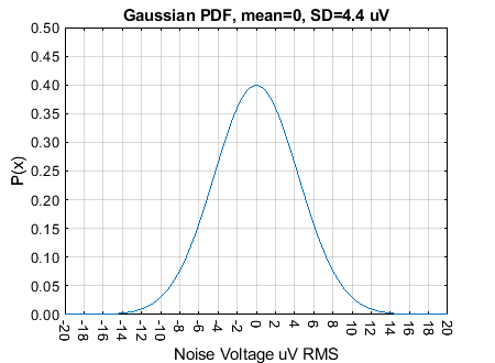
Looking again at the classic Gaussian PDF in Figure 3-2, also known as a normal distribution or bell curve because of its resemblance to the shape of a traditional bell, there are some interesting features. The probability of a noise voltage being between, say \(x_1\) and \(x_2\), \(p(x_1 \le x \le x_2) \), would be the area under the curve between \(x_1\) and \(x_2\). (3-5).

\[p (x_1 \le x \le x_2) = \int_{x_1}^{x_1} p(x) dx \]

Applying the Auto-correlation Function to AWGN Noise Samples

Further to the comments in Section 2, another way of understanding use of the term 'white' in AWGN is to apply the Auto Correlation Function (ACF) followed by a Fourier transform to convert the result from the time domain to a power against frequency spectrum [6] [7].

The individual charges which generate AWGN voltages are in large numbers, random and independent. Therefore, AWGN is the result of a random process. Then by applying the ACF to a sampled AWGN voltage against time waveform, the result is a delta function of the time difference (\( \tau \)) with a weighting of \(N_0 / 2 \) where \(N_0\) is the noise power density in watts/hertz, \(W / Hz\). (4-1).

\[ \begin{align} R_N (\tau) &= E \left[ N(t) \, N(t+\tau) \right] \\ &= \frac{N_0}{2} \delta(\tau) \\ \end{align} \]

The symbols used in (4-1) are:

• \(R_N (\tau) \): the auto correlation function of \(\tau\).
• \(N(t)\): the AWGN voltage as a function of time \(t\).
• \(N_0 \): the AWGN power spectral density in watts per hertz \(W / Hz\).
• \(E [ \,\, ] \): the expected or mean value.

In (4-1), the weighting of the delta function is divided by 2 to relate to the power on each side of a double sideband frequency spectrum, covering both positive and negative frequencies. For a single sided spectrum the weighting would be \(N_0\).

• Return to Top
• Return to Chris Angove's Home Page